Estimating Cross-Platform Usage Structure from Large-Scale Marginal Distributions and a Small Panel

Suppose there are two video services, A and B. We know the usage-time distribution for each service, including the share of people who use A for at least five hours per week and the corresponding share for B. These data alone, however, do not reveal how many people use both services for at least five hours per week. That calculation requires not only the marginal distribution of each service but also information about how the same individuals divide their time between the two.

If large-scale service logs could be linked at the individual level through a common identifier, the overlap could be counted directly. In practice, population-scale linkage is not always feasible because of constraints involving identity spaces, units of measurement, consent, and intercompany data sharing. At the same time, each service’s usage-time distribution may be measured accurately from large-scale logs, while a smaller single-source panel may observe both services for the same people. One example is survey data collected from consenting users about their activity across multiple video services.

Using simulated data, this article combines large-scale logs and a small panel through a Gaussian copula to estimate overlap and complementarity in usage intensity among users of both services. For simplicity, every person in the analysis is assumed to have positive usage time for both A and B. The target is therefore overlap in usage intensity, not whether each service is used at all.

Audience overlap beyond marginal distributions

Let \(X\) and \(Y\) denote weekly usage time for services A and B. Even if large-scale logs identify the marginal distributions

\[ F_X(x) = P(X \leq x), \qquad F_Y(y) = P(Y \leq y) \]

the joint distribution \(F_{XY}(x,y)\) is not uniquely determined. For example, even if 20% of people use A for at least five hours per week and 20% do the same for B, the share of heavy users of both services depends greatly on whether those two groups contain mostly the same people or mostly different people.

The simplest assumption is independence, which gives

\[ P(X \geq 5, Y \geq 5) = P(X \geq 5)P(Y \geq 5) \]

However, if available time, interest in video, and daily routines affect usage of both services, the independence assumption will tend to underestimate overlap.

Another option is to estimate overlap directly from the small panel. Error becomes large, however, for combinations represented by few panelists. The estimate also inherits any discrepancy between the panel’s usage-time distribution and that of the population.

Separation of marginal distributions and dependence with a copula

A copula expresses the joint distribution as

\[ F_{XY}(x,y) = C_\theta\!\left( F_X(x), F_Y(y) \right) \]

where \(F_X\) and \(F_Y\) are the service-specific usage-time distributions and \(C_\theta\) is their dependence structure. This decomposition assigns a distinct role to each data source.

Quantity	Data source	Information supplied by the data
\(F_X\)	Large-scale logs for service A	Usage-time distribution for A
\(F_Y\)	Large-scale logs for service B	Usage-time distribution for B
\(C_\theta\)	Small panel observing the same individuals	Rank dependence between A and B

This article uses a Gaussian copula for the dependence structure, implemented with the {copula} package.

A Gaussian copula assigns correlation \(\rho\) to latent standard normal variables \((Z_X,Z_Y)\):

\[ (Z_X,Z_Y) \sim N\!\left( \begin{bmatrix}0 \\ 0\end{bmatrix}, \begin{bmatrix}1 & \rho \\ \rho & 1\end{bmatrix} \right) \]

When \(\rho = 0\), the services are independent. When \(\rho > 0\), people with a high usage rank for one service also tend to rank highly for the other. This model does not assume that usage time itself is normally distributed. Skewed distributions and differences in shape between services are handled by \(F_X\) and \(F_Y\).

Dependence estimation from a small panel

Let the panel size be \(n\). Usage times are ranked within the panel and divided by \(n + 1\), preventing values of exactly 0 or 1.

\[ U_i = \frac{\operatorname{rank}(X_i)}{n + 1}, \qquad V_i = \frac{\operatorname{rank}(Y_i)}{n + 1} \]

The ranks are then transformed into normal scores, and their correlation is estimated.

\[ Z_{Xi} = \Phi^{-1}(U_i), \qquad Z_{Yi} = \Phi^{-1}(V_i), \qquad \hat\rho = \operatorname{Cor}(Z_X,Z_Y) \]

The key distinction is that within-panel ranks are used to estimate dependence, whereas the marginal distributions from the large-scale logs map probabilities back to usage times. Applying the population CDF directly to observations from a biased panel would not produce uniform pseudo-observations. Using within-panel ranks does not, however, eliminate selection bias. This limitation is examined later.

Combining the estimated \(\hat\rho\) with the marginal distributions from large-scale logs yields overlap estimates for any threshold. For example,

\[ \begin{aligned} P(X \geq 5,Y \geq 5) = {} & 1 - F_X(5) - F_Y(5) \\ & +C_{\hat\rho}\!\left( F_X(5),F_Y(5) \right) \end{aligned} \]

Once the joint distribution has been estimated through a copula, thresholds such as at least three or ten hours per week can be changed after estimation. The model therefore supports a richer range of downstream analyses than a single precomputed overlap statistic.

Simulation design

Usage-time generation from a shared viewing propensity

The population contains 500,000 people. A shared factor \(H_i\) represents each person’s propensity to watch video, and weekly usage times are generated as follows.

\[ \log X_i = \log 2 + 0.8H_i + \varepsilon_{Ai}, \qquad \varepsilon_{Ai} \sim N(0,0.6^2) \]

\[ \log Y_i = \log 1.5 + 0.6H_i + \varepsilon_{Bi}, \qquad \varepsilon_{Bi} \sim N(0,0.8^2) \]

The error terms are mutually independent and independent of \(H_i\). The latent factor summarizes hypothetical characteristics such as interest in video, available leisure time, and viewing habits. Conditional on \(H_i = 0\), median weekly usage is two hours for A and 1.5 hours for B.

The main simulation uses a mixture in which 20% of the population has a somewhat higher viewing propensity.

\[ B \sim \operatorname{Bernoulli}(0.2), \qquad Z_H \sim N(0,1), \qquad B \perp \!\!\! \perp Z_H \]

The variable \(B\) is a switch selecting the mixture component. When \(B = 0\), a person belongs to the group with the baseline viewing propensity. When \(B = 1\), the person belongs to a group whose mean is 1.5 higher. The latent usage propensity is generated as follows.

\[ H_{\mathrm{raw}} = 1.5B + Z_H, \qquad H = \frac{H_{\mathrm{raw}} - 0.3}{\sqrt{1.36}} \]

The marginal distribution of \(H_{\mathrm{raw}}\) is therefore \(0.8N(0,1) + 0.2N(1.5,1)\). Here, 1.5 is a simulation parameter controlling the separation between the two groups. Because \(E[H_{\mathrm{raw}}] = 0.3\) and \(\operatorname{Var}(H_{\mathrm{raw}}) = 1.36\), \(H\) is standardized to mean 0 and variance 1. Its distribution remains nonnormal, making the Gaussian copula intentionally misspecified as an approximation in this mixture scenario.

If instead \(H \sim N(0,1)\), then \((\log X,\log Y)\) follows a bivariate normal distribution and its true dependence structure corresponds exactly to a Gaussian copula. The evaluation focuses on the mixture scenario to assess approximation performance under more demanding conditions.

set.seed(20260907)

n_population <- 500000
n_panel <- 1000
n_rep <- 100
heavy_thresholds <- c(3, 5, 10)
light_threshold <- 1

population <- tibble(
  b = rbinom(n_population, 1, 0.2),
  z_h = rnorm(n_population, mean = 0, sd = 1),
  eps_x = rnorm(n_population, mean = 0, sd = 0.6),
  eps_y = rnorm(n_population, mean = 0, sd = 0.8)
) |>
  mutate(
    h_raw = 1.5 * b + z_h,
    h = (h_raw - 0.3) / sqrt(1.36),
    x = exp(log(2) + 0.8 * h + eps_x),
    y = exp(log(1.5) + 0.6 * h + eps_y),
    sampling_weight = 0.5 + 0.4 * plogis(1.5 * h)
  )

rho_population <- population |>
  summarise(
    rho = cor(
      qnorm(rank(x) / (n() + 1)),
      qnorm(rank(y) / (n() + 1))
    )
  ) |>
  pull(rho)

population_summary <- population |>
  select(x, y) |>
  cross_join(tibble(heavy = heavy_thresholds)) |>
  mutate(
    a_heavy = x >= heavy,
    b_heavy = y >= heavy,
    a_light = x < light_threshold,
    b_light = y < light_threshold
  ) |>
  summarise(
    fx_h = mean(!a_heavy),
    fy_h = mean(!b_heavy),
    fx_l = mean(a_light),
    fy_l = mean(b_light),
    both_heavy = mean(a_heavy & b_heavy),
    a_heavy_b_light = mean(a_heavy & b_light),
    a_light_b_heavy = mean(a_light & b_heavy),
    .by = heavy
  ) |>
  pivot_longer(
    c(both_heavy, a_heavy_b_light, a_light_b_heavy),
    names_to = "metric",
    values_to = "truth"
  )

panels <- tibble(rep = seq_len(n_rep)) |>
  mutate(
    panel = map(rep, \(.) {
      population |>
        slice_sample(n = n_panel, weight_by = sampling_weight)
    })
  ) |>
  unnest(panel) |>
  mutate(
    u = rank(x) / (n() + 1),
    v = rank(y) / (n() + 1),
    rho_panel = cor(qnorm(u), qnorm(v)),
    panel_h_mean = mean(h),
    .by = rep
  )

panel_summary <- panels |>
  select(rep, x, y, rho_panel, panel_h_mean) |>
  cross_join(tibble(heavy = heavy_thresholds)) |>
  mutate(
    a_heavy = x >= heavy,
    b_heavy = y >= heavy,
    a_light = x < light_threshold,
    b_light = y < light_threshold
  ) |>
  summarise(
    both_heavy = mean(a_heavy & b_heavy),
    a_heavy_b_light = mean(a_heavy & b_light),
    a_light_b_heavy = mean(a_light & b_heavy),
    rho_panel = first(rho_panel),
    panel_h_mean = first(panel_h_mean),
    .by = c(rep, heavy)
  ) |>
  pivot_longer(
    c(both_heavy, a_heavy_b_light, a_light_b_heavy),
    names_to = "metric",
    values_to = "direct"
  )

simulation_raw <- panel_summary |>
  left_join(population_summary, by = c("heavy", "metric")) |>
  mutate(
    copula_u = if_else(metric == "a_light_b_heavy", fx_l, fx_h),
    copula_v = if_else(metric == "a_heavy_b_light", fy_l, fy_h)
  ) |>
  mutate(
    cdf_panel = copula::pCopula(
      cbind(copula_u, copula_v),
      copula::normalCopula(
        param = first(rho_panel),
        dim = 2,
        dispstr = "un"
      )
    ),
    .by = rep
  ) |>
  mutate(
    cdf_population = copula::pCopula(
      cbind(copula_u, copula_v),
      copula::normalCopula(
        param = rho_population,
        dim = 2,
        dispstr = "un"
      )
    ),
    cdf_base = case_when(
      metric == "both_heavy" ~ 1 - fx_h - fy_h,
      metric == "a_heavy_b_light" ~ fy_l,
      metric == "a_light_b_heavy" ~ fx_l
    ),
    cdf_sign = if_else(metric == "both_heavy", 1, -1),
    independence = cdf_base + cdf_sign * copula_u * copula_v,
    fusion = cdf_base + cdf_sign * cdf_panel,
    oracle = cdf_base + cdf_sign * cdf_population
  ) |>
  select(
    rep,
    heavy,
    metric,
    truth,
    independence,
    direct,
    fusion,
    oracle,
    rho_panel,
    panel_h_mean
  )

simulation_long <- simulation_raw |>
  pivot_longer(
    c(independence, direct, fusion, oracle),
    names_to = "method",
    values_to = "estimate"
  )

simulation_summary <- simulation_long |>
  summarise(
    truth = first(truth),
    mean_estimate = mean(estimate),
    bias_pp = 100 * mean(estimate - truth),
    sd_pp = 100 * sd(estimate),
    rmse_pp = 100 * sqrt(mean((estimate - truth)^2)),
    .by = c(heavy, metric, method)
  )

Large-scale marginal data and a small panel

For each service, the empirical distribution of the full population of 500,000 is used as the large-scale dataset. The marginal distributions are therefore treated as nearly known in this simulation. By contrast, the panel that observes both \(X\) and \(Y\) for the same people contains only 1,000 individuals.

The panel is a biased sample in which people with a higher shared viewing propensity \(H\) are more likely to be selected. The relative sampling weight is

\[ w(H) = 0.5 + 0.4\operatorname{logit}^{-1}(1.5H) \]

This is a relative weight used for sampling without replacement, not each person’s inclusion probability. The panel’s marginal distributions differ from those of the population, while the change in its dependence structure remains small under this design. The setup is not robust to every form of selection bias.

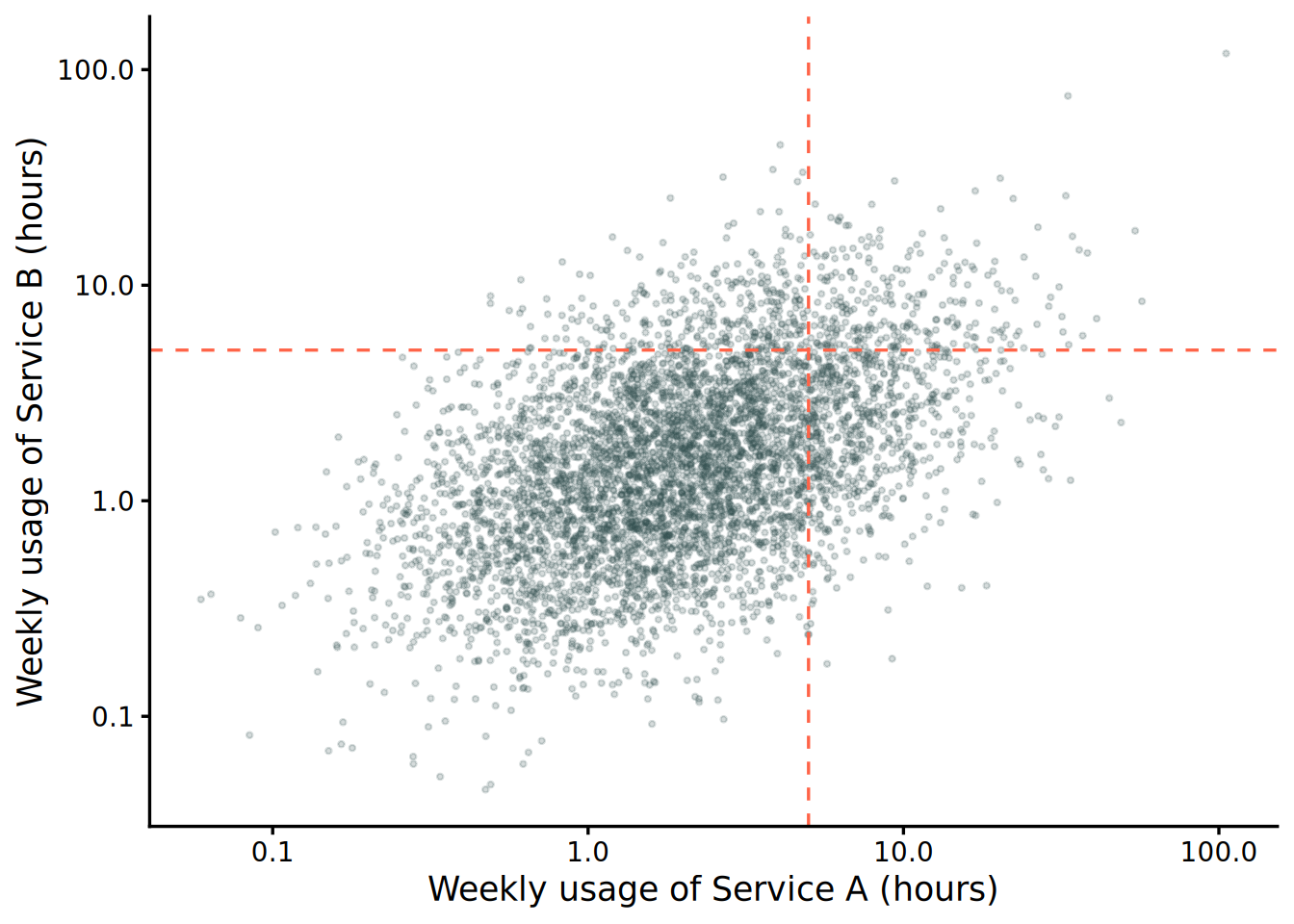
Figure 1: Weekly usage times for 5,000 people sampled from the nonnormal viewing-propensity mixture. Positive dependence between the two services induced by a shared viewing propensity.

Comparison of estimation methods

Five quantities are compared using the same panel samples.

1. Direct aggregation over the population, which is the simulation truth.
2. An independence estimate using the large-scale marginal distributions.
3. Direct aggregation over the panel of 1,000 people.
4. Gaussian copula fusion using the large-scale marginal distributions and within-panel ranks.
5. A Gaussian approximation with \(\rho\) estimated from the full population. This diagnostic benchmark isolates model error but is unavailable in practice because it uses population-level joint information.

Heavy-user thresholds are set at 3, 5, and 10 hours per week, while a light user is defined as someone with less than one hour per week. Three probabilities are evaluated.

• Both heavy: \(P(X \geq h,Y \geq h)\)
• A heavy and B light: \(P(X \geq h,Y < 1)\)
• A light and B heavy: \(P(X < 1,Y \geq h)\)

Holding the population fixed, panel sampling is repeated 100 times. The evaluation reports the truth, mean estimate, bias, standard deviation, and root mean squared error (RMSE). Error metrics are expressed in percentage points (pp).

Results for the viewing-propensity mixture

The analysis begins with the most practice-oriented scenario, which combines mild nonnormality with biased panel sampling. Table 1 reports results for a heavy-user threshold of five hours per week.

Table 1: Estimation performance for the viewing-propensity mixture, biased panel, and five-hour heavy-user threshold. Bias, standard deviation, and RMSE in pp.

Method	Truth	Mean estimate	Bias	SD	RMSE
A heavy / B light
Independence assumption	1.913%	6.155%	4.242	0.000	4.242
Direct panel estimate	1.913%	2.075%	0.162	0.489	0.513
Gaussian copula fusion	1.913%	2.013%	0.100	0.173	0.199
A light / B heavy
Independence assumption	0.543%	2.838%	2.295	0.000	2.295
Direct panel estimate	0.543%	0.521%	−0.022	0.224	0.224
Gaussian copula fusion	0.543%	0.564%	0.021	0.073	0.076
Both heavy
Independence assumption	5.408%	2.046%	−3.362	0.000	3.362
Direct panel estimate	5.408%	6.630%	1.222	0.847	1.484
Gaussian copula fusion	5.408%	5.138%	−0.270	0.188	0.329

For the both-heavy outcome, the independence assumption produces a large error because it ignores the positive dependence induced by the shared viewing propensity. Gaussian copula fusion, by contrast, has lower RMSE than direct panel aggregation.

The fusion estimator also has lower RMSE for the A-heavy/B-light and A-light/B-heavy outcomes. Using marginal distributions from large-scale data stabilizes estimation relative to counting rare combinations directly in the small panel.

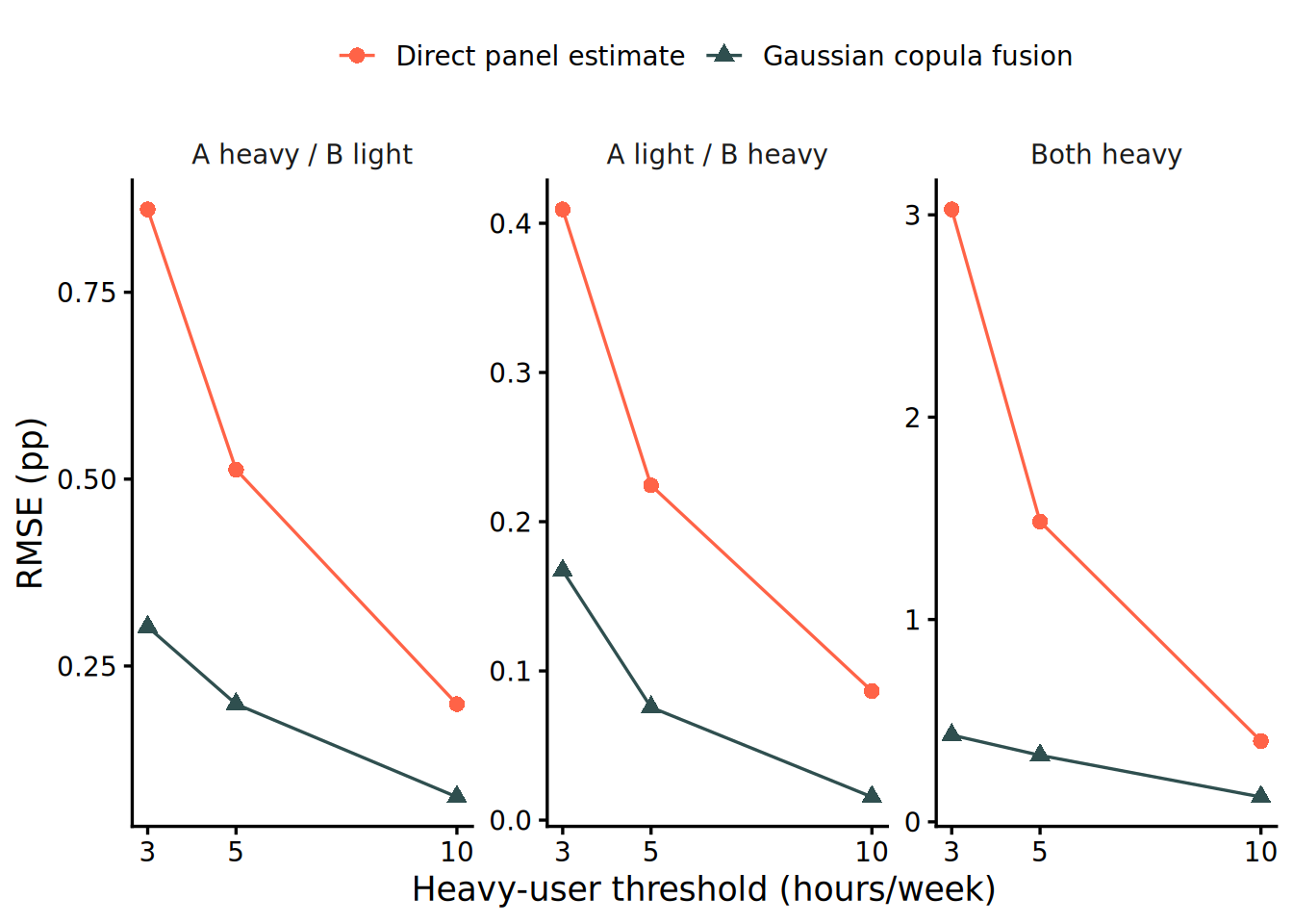
Figure 2: RMSE for the nonnormal viewing-propensity mixture and biased panel. One-hour light-user threshold, heavy-user threshold on the horizontal axis, pp on the vertical axis.

Figure 2 compares direct panel aggregation with fusion across all three heavy-user thresholds. In the viewing-propensity mixture, fusion has lower RMSE for every threshold and outcome.

Sources of the accuracy gain

The main advantage of fusion is that it does not require the panel of 1,000 people to estimate every component. In direct panel aggregation, for example, the estimate for at least five hours on both A and B is supported only by panelists in that cell. As the target combination becomes rarer, the effective sample size falls and the estimate becomes more variable.

With copula fusion, the panel is used mainly to estimate a single dependence parameter, \(\rho\). The shares above five hours and below one hour for each service come from the marginal distributions of 500,000 people. The matched-person information in the panel is therefore concentrated on estimating dependence, while large-scale data replace the panel’s sampling error and bias in the margins.

This account applies only when a simple dependence model approximates the usage structure sufficiently well. Accuracy improves even in the viewing-propensity mixture, where the Gaussian copula is approximate, because the dependence captured by the normal-score correlation changes little between the biased panel and the population.

Required assumptions

Transportability of the dependence structure from panel to population

Let \(S = 1\) indicate panel participation. The central assumption is

\[ C_{X,Y \mid S=1} \approx C_{X,Y} \]

The relationship between usage of the two services among panelists must be approximately the same in the population.

In this simulation, people who watch more video are more likely to be selected. This shifts the panel’s usage-time distributions but leaves rank dependence between the services nearly unchanged. The results therefore support only the narrower claim that fusion works when the margins are biased but the dependence structure is preserved.

For example, if people who prefer only A are more likely to join the panel while those who prefer only B are less likely, selection changes the dependence structure itself. Supplying correct marginal distributions from large-scale logs cannot repair a misspecified copula in that case. Additional designs are needed to assess transportability, such as dependence estimation by covariate group, calibration weighting, or comparisons across multiple panels.

Consistency of measurement definitions

The marginal data and the panel must measure the same estimand.

• The observation window is the same weekly period.
• Usage time is defined consistently.
• Person-level and device-level units are not mixed.
• Background playback and similar events are handled consistently.

A copula addresses dependence, not measurement error or a mismatch in estimands. Combining datasets that measure different constructs does not resolve that inconsistency.

Adequacy of the Gaussian copula approximation

A Gaussian copula represents dependence through a single correlation parameter. It is convenient as a baseline model and extends naturally to a correlation matrix for multiple platforms, but it cannot represent every dependence structure.

If heterogeneous groups such as both light, both heavy, A-focused, and B-focused users coexist, the local overlap structure can differ even under the same overall correlation. A Gaussian copula also has no asymptotic tail dependence. If extreme outcomes matter, such as the probability that the top 1% of users overlap across both services, a t copula may be a better candidate.

For the ordinary segment thresholds of 3, 5, and 10 hours per week in this article, the Gaussian copula serves as the baseline model. Model selection should consider not only overall fit but also how well each candidate reproduces the overlap metrics that will ultimately be used.

Zero usage in real-world data

Real weekly data often contain many zero-hour observations from nonusers, creating extensive rank ties. A rank transformation that assumes continuous distributions should not be applied unchanged. Instead, usage incidence and positive usage time among users should be estimated separately. The former captures discrete outcomes such as neither service and A only, while the latter models dependence between positive usage times.

Discussion

Marginal distributions alone are not sufficient to determine cross-platform audience overlap.

One possible approach is to combine large-scale service logs with a smaller single-source panel: the former can be used to estimate the marginal distributions, while the latter provides information about dependence between the services.

In this simulation, Gaussian copula fusion gave more stable overlap estimates than direct aggregation from the small panel.

Whether this works in practice depends on the assumptions. In particular, the dependence structure estimated from the panel needs to be reasonably representative of the target population, and the data sources need to measure compatible quantities. Copula fusion should therefore be viewed as one possible data-fusion approach rather than a general solution to selection bias or measurement mismatch.