| Segment | \(n\) | Impressions | Reached | Mean FQ | Variance |
|---|---|---|---|---|---|
| Light | 799,921 | 79,655 | 65,846 | 0.10 | 0.13 |
| Heavy | 200,079 | 602,701 | 150,283 | 3.01 | 12.05 |
A frequency distribution records how many times each user was exposed to an ad during a campaign. In streaming advertising, this distribution is the input to reach and frequency planning: given a target number of impressions, how many unique users will see the ad at least once?
The distribution has a characteristic shape. Most users in the target population receive zero impressions. Among those reached, the number of users drops sharply from one exposure to two, then continues to decline along a long right tail produced by a small number of heavy viewers. A Poisson distribution cannot reproduce this shape: its variance equals its mean, but empirical frequency distributions are overdispersed, often by an order of magnitude. The negative binomial distribution handles overdispersion through an extra parameter, but a single negative binomial still fails to reproduce the shape that arises when the population contains distinct viewing segments: a sharp spike near zero from light viewers and a heavy tail from heavy viewers cannot be matched by a single dispersion parameter.
This post fits a finite mixture of negative binomial distributions to a simulated frequency distribution using the EM algorithm (via the flexmix package), and derives a reach curve from the estimated parameters.
The negative binomial as a Poisson-Gamma mixture
A natural model for ad exposure counts starts with the Poisson distribution. If user \(i\) has a constant exposure rate \(\lambda_i\) over the campaign period, the number of impressions is \(X_i \mid \lambda_i \sim \text{Poisson}(\lambda_i)\).
In a heterogeneous population, \(\lambda_i\) varies across users. A conjugate model places a Gamma prior on the rate:
\[ \lambda_i \sim \text{Gamma}\!\left( \theta, \; \frac{\theta}{\mu} \right) \]
where \(\mu = E[\lambda_i]\) is the population mean rate and \(\theta > 0\) controls the dispersion. The Gamma is parameterized so that \(E[\lambda_i] = \mu\) and \(\text{Var}(\lambda_i) = \mu^2 / \theta\).
Marginalizing over \(\lambda_i\):
\[ P(X = x) = \int_0^{\infty} \frac{e^{-\lambda}\lambda^x}{x!} \cdot \frac{(\theta/\mu)^{\theta}}{\Gamma(\theta)} \lambda^{\theta-1} e^{-\theta\lambda/\mu} \, d\lambda \]
The integral evaluates to the negative binomial probability mass function:
\[ P(X = x) = \binom{x + \theta - 1}{x} \left( \frac{\theta}{\theta + \mu} \right)^{\!\theta} \left( \frac{\mu}{\theta + \mu} \right)^{\!x}, \quad x = 0, 1, 2, \dots \]
The moments are:
\[ E[X] = \mu, \quad \text{Var}(X) = \mu + \frac{\mu^2}{\theta} \]
The \(\mu^2/\theta\) term is the excess variance from population heterogeneity. As \(\theta \to \infty\), \(\text{Var}(\lambda_i) \to 0\), the population becomes homogeneous, and the negative binomial converges to the Poisson. Small \(\theta\) means high heterogeneity and heavy overdispersion.
This parameterization (mean \(\mu\), dispersion \(\theta\)) is used by glmmTMB::nbinom2 in R and matches the convention throughout this post.
Finite mixture of negative binomials
A single negative binomial assumes one Gamma-distributed rate across the entire population. If the population contains structurally distinct segments (light viewers who rarely see ads and active viewers who consume more content), a single Gamma cannot represent the bimodal rate distribution that results.
A finite mixture model partitions the population into \(K\) latent segments. User \(i\) belongs to segment \(k\) with probability \(\pi_k\), and given segment \(k\), the exposure count follows a segment-specific negative binomial:
\[ P(X = x) = \sum_{k=1}^{K} \pi_k \cdot \text{NB}(x \mid \mu_k, \theta_k) \]
where \(\sum_{k=1}^{K} \pi_k = 1\) and each component has its own mean \(\mu_k\) and dispersion \(\theta_k\). The model has \(3K - 1\) free parameters: \(K\) means, \(K\) dispersions, and \(K - 1\) mixing proportions.
The parameters are estimated by the EM algorithm. The E-step computes posterior segment membership probabilities for each observation; the M-step re-estimates \((\pi_k, \mu_k, \theta_k)\) by weighted maximum likelihood within each segment. The flexmix package (Grün and Leisch 2008) implements this procedure for general finite mixture models. With the countreg::FLXMRnegbin driver, it can fit mixtures of negative binomial distributions directly.
The number of components \(K\) is selected by BIC. Adding components always improves log-likelihood; BIC penalizes the additional parameters and identifies the point where added complexity no longer improves fit.
Simulation
Data generation
The simulation creates a population of \(N = 1{,}000{,}000\) users drawn from two segments. The parameters reflect a typical frequency distribution in digital advertising: a large light segment that accounts for most of the population, and a smaller heavy segment with higher mean exposure and lower relative dispersion.
| Segment | \(\pi\) | \(\mu\) | \(\theta\) |
|---|---|---|---|
| Light | 0.80 | 0.1 | 0.3 |
| Heavy | 0.20 | 3.0 | 1.0 |
The heavy segment has both a higher mean (\(\mu = 3.0\) vs. \(0.1\)) and a higher \(\theta\) (\(1.0\) vs. \(0.3\)): active viewers see more ads, while their exposure rates are less heterogeneous relative to their mean. The variance within each segment is \(\mu + \mu^2/\theta\): \(0.13\) for light, \(12.0\) for heavy.
The observed mean frequencies match the population parameters. The variance column confirms the overdispersion: the heavy segment’s variance (\(\approx 12\)) is four times its mean (\(\approx 3\)), consistent with \(\mu + \mu^2/\theta = 3 + 9/1 = 12\).
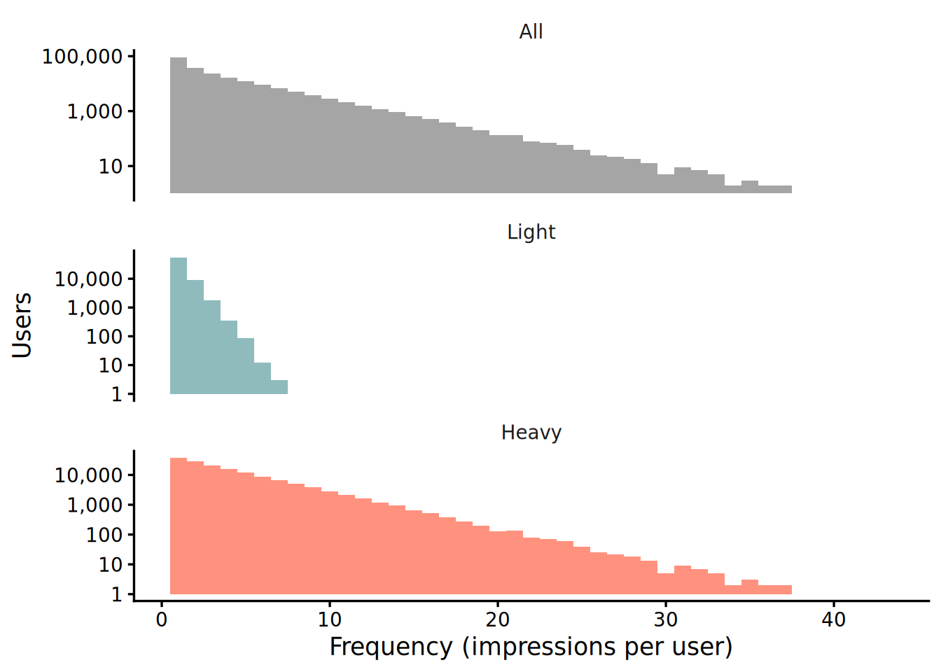
The aggregate distribution (top panel) shows the characteristic shape: a sharp peak at \(FQ = 1\), rapid decay, and a long right tail. The component panels show how this shape arises from the superposition of two distributions with different means.
In practice, only the aggregate distribution is observed. The per-segment breakdown is unknown. The mixture model’s task is to recover this latent segment structure from the aggregate counts alone.
Fitting a single negative binomial
As a baseline, fit a single negative binomial to the aggregate frequency distribution using glmmTMB. The weights argument accepts frequency counts, allowing the model to use the aggregated table \((x, \text{count})\) directly.
| \(\hat{\mu}\) | \(\hat{\theta}\) |
|---|---|
| 0.682 | 0.135 |
The estimated \(\hat{\mu}\) correctly recovers the population mean (\(\sum \pi_k \mu_k = 0.80 \times 0.1 + 0.20 \times 3.0 = 0.68\)). The estimated \(\hat{\theta}\) is far below the true within-segment values (\(0.3\) and \(1.0\)). A single negative binomial must absorb both within-segment overdispersion and between-segment heterogeneity into one \(\theta\) parameter, forcing it artificially low.
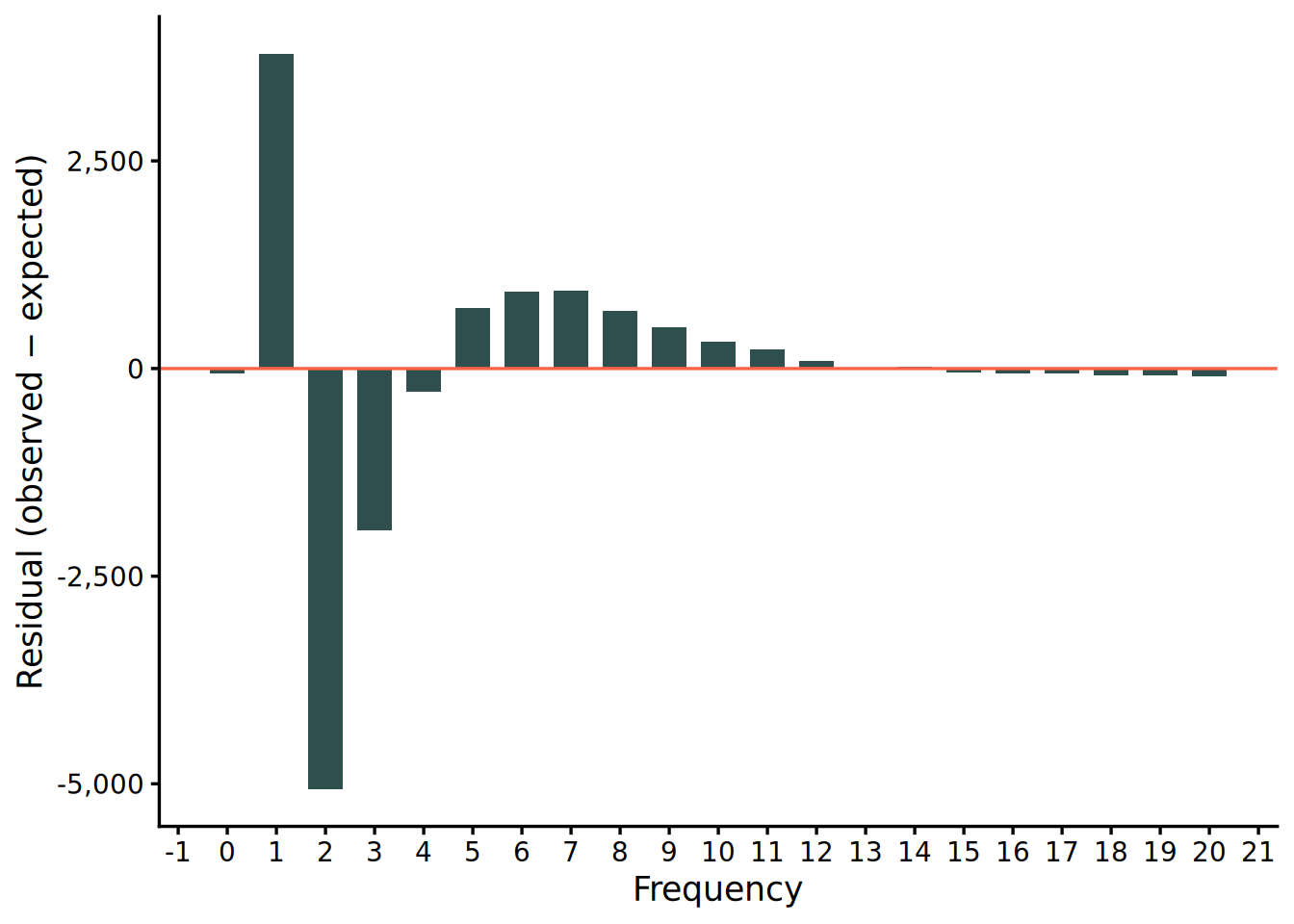
The residual plot confirms the misfit. The single negative binomial systematically underpredicts at low frequencies and overpredicts at moderate frequencies. The model cannot simultaneously match the sharp peak driven by the light segment and the heavy tail driven by the heavy segment.
Fitting the mixture model
Fit finite mixtures with \(K = 2, 3, 4\) components using flexmix::stepFlexmix with the countreg::FLXMRnegbin driver. The nrep = 50 argument runs 50 random initializations per \(K\) to mitigate the EM algorithm’s sensitivity to starting values.
| \(K\) | BIC |
|---|---|
| 2 | 1,877,747 |
| 3 | 1,877,788 |
| 4 | 1,877,829 |
\(K = 2\) achieves the lowest BIC. Additional components do not improve fit enough to justify the added parameters.
| Segment |
True
|
Estimated
|
||||
|---|---|---|---|---|---|---|
| \(\pi\) | \(\mu\) | \(\theta\) | \(\hat{\pi}\) | \(\hat{\mu}\) | \(\hat{\theta}\) | |
| Light | 0.800 | 0.100 | 0.300 | 0.803 | 0.104 | 0.274 |
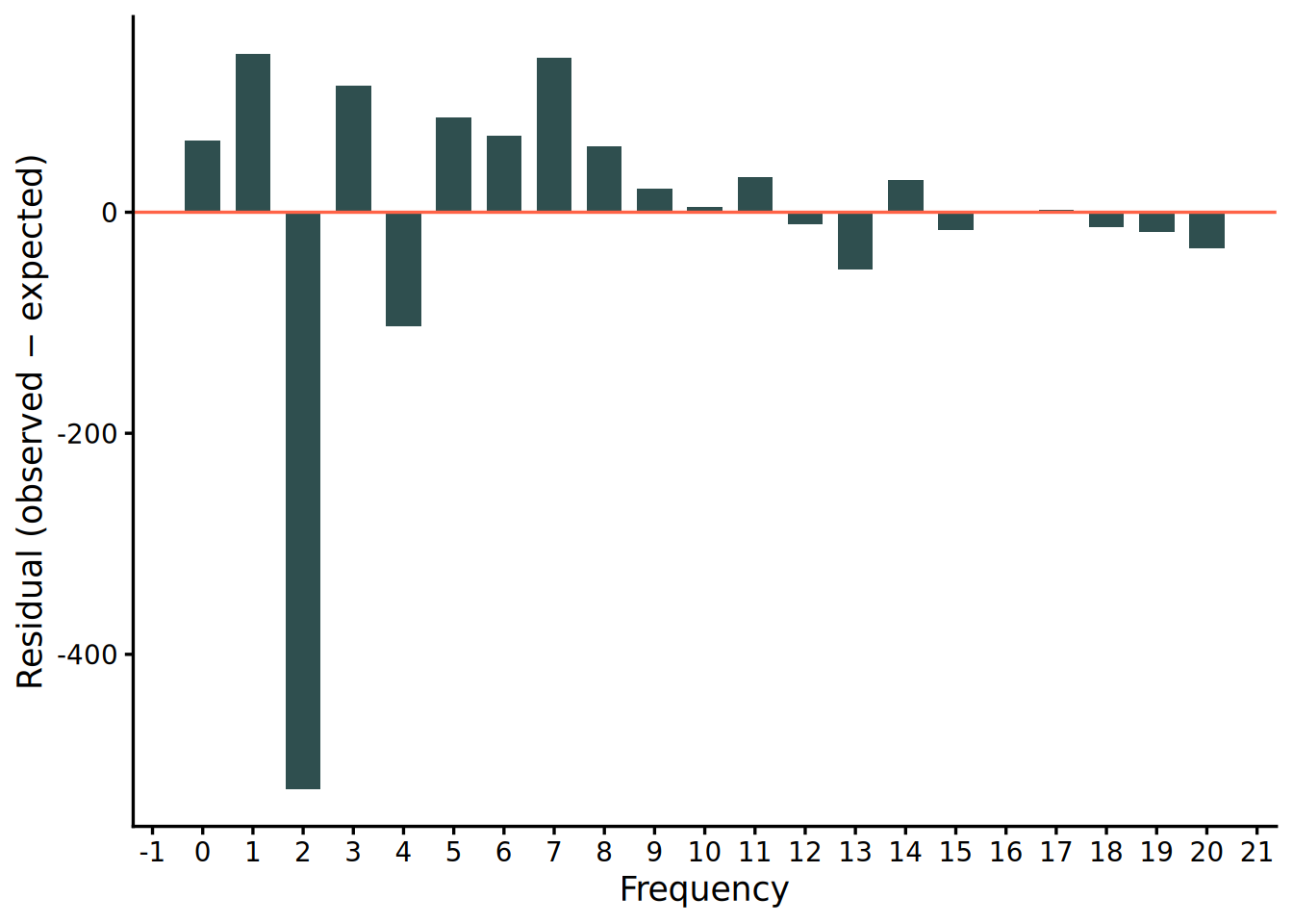
| Heavy | 0.200 | 3.000 | 1.000 | 0.197 | 3.038 | 1.003 |
The recovery table matches each estimated component to its nearest true segment by \(\mu\). With a 30-fold gap between the two segment means (\(\mu = 0.1\) vs. \(3.0\)), the EM algorithm has no difficulty separating the components.
From mixture parameters to reach curves
Reach as a function of the mixture
Reach is the number of users with at least one impression. Under the mixture model, the probability of zero impressions is:
\[ P(X = 0) = \sum_{k=1}^{K} \pi_k \cdot P(X = 0 \mid \mu_k, \theta_k) \]
The negative binomial zero probability has a closed form:
\[ P(X = 0 \mid \mu, \theta) = \left( \frac{\theta}{\theta + \mu} \right)^{\!\theta} \]
The reach rate is \(1 - P(X = 0)\), and the reach count in a population of size \(N\) is:
\[ \text{Reach} = N \left[ 1 - \sum_{k=1}^{K} \pi_k \left( \frac{\theta_k}{\theta_k + \mu_k} \right)^{\!\theta_k} \right] \]
Scaling to different impression levels
The estimated \(\mu_k\) values correspond to the observed total impressions \(I_{\text{obs}}\). To predict reach at a different impression level \(I_{\text{target}}\), scale each component mean proportionally:
\[ \mu_k' = \frac{I_{\text{target}}}{I_{\text{obs}}} \cdot \mu_k \]
This assumes that increasing the total number of impressions by a factor \(s\) increases each user’s expected exposure by the same factor. The assumption holds when the additional impressions are distributed across the population in the same relative proportions as in the original campaign. It does not hold if the additional impressions are concentrated on specific segments (e.g., retargeting only heavy viewers).
Substituting \(\mu_k'\) into the reach formula produces a reach curve: reach as a function of total impressions.
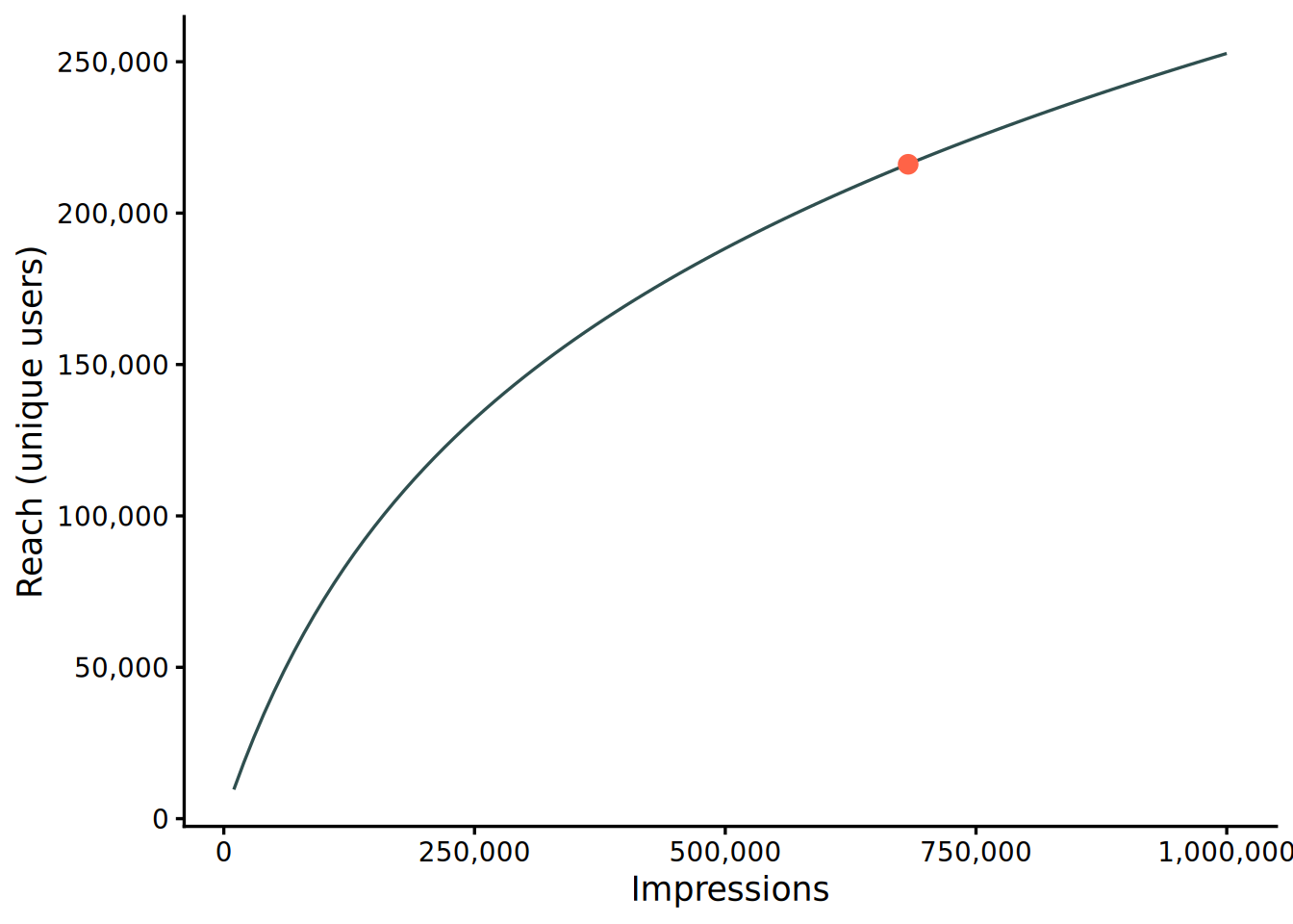
The curve passes through the observed data point, confirming internal consistency. The concavity reflects diminishing returns: as impressions increase, a growing share is absorbed by heavy viewers who have already been reached, producing less incremental reach per impression. The mixture model captures this structure because the heavy segment’s high \(\mu\) concentrates repeated exposures on a small fraction of users.
R code
library(tidyverse)

# --- Simulation ---

simulate_frequency <- function(n_population, params) {
  params |>
    slice_sample(n = n_population, weight_by = prior, replace = TRUE) |>
    mutate(
      user_id = row_number(),
      imp = rnbinom(n(), mu = mu, size = theta)
    )
}

true_params <- tribble(
  ~component , ~prior , ~mu , ~theta ,
  "Light"    , 0.80   , 0.1 , 0.3    ,
  "Heavy"    , 0.20   , 3.0 , 1.0    ,
)

set.seed(42)
sim_data <- simulate_frequency(1000000, true_params)
freq_dist <- sim_data |> count(imp, name = "cnt")


# --- Single NB fit ---

fit_single <- glmmTMB::glmmTMB(
  data = freq_dist,
  formula = imp ~ 1,
  family = glmmTMB::nbinom2,
  weights = cnt
)

single_mu <- exp(glmmTMB::fixef(fit_single)$cond[["(Intercept)"]])
single_theta <- glmmTMB::sigma(fit_single)


# --- Mixture NB fit ---

set.seed(42)
fit_mix <- flexmix::stepFlexmix(
  data = freq_dist,
  formula = imp ~ 1,
  k = 2:4,
  model = countreg::FLXMRnegbin(),
  weights = ~cnt,
  control = list(iter.max = 1000, minprior = 0.05),
  nrep = 50,
  verbose = FALSE
)

# BIC comparison
sapply(fit_mix@models, BIC)

# Extract best model parameters
fit_best <- flexmix::getModel(fit_mix, which = "BIC")

mix_params <- flexmix::parameters(fit_best) |>
  t() |>
  as_tibble() |>
  rename(log_mu = `coef.(Intercept)`) |>
  mutate(
    component = row_number(),
    prior = flexmix::prior(fit_best),
    mu = exp(log_mu),
    .before = 1
  ) |>
  arrange(mu)


# --- Reach curve ---

reach_from_mixture <- function(target_imp, params_df, total_uu, observed_imp) {
  s <- target_imp / observed_imp
  p_zero <- params_df |>
    mutate(
      scaled_mu = mu * s,
      p0 = prior * dnbinom(0, mu = scaled_mu, size = theta)
    ) |>
    summarise(p0 = sum(p0)) |>
    pull(p0)
  total_uu * (1 - p_zero)
}

total_uu <- sum(freq_dist$cnt)
observed_imp <- sum(freq_dist$imp * freq_dist$cnt)

# Predict reach at 500,000 impressions
reach_from_mixture(500000, mix_params, total_uu, observed_imp)