Suppose a media planner asks, “How many unique users watched either K-Drama or Romance in the past 90 days?” Here, unique users (UU) refers to the number of distinct people who satisfy the conditions, with each person counted only once. This number helps determine whether the proposed targeting segment can support the planned campaign budget.
With access to the complete viewing logs, the qualifying viewers could be counted directly. Repeatedly scanning a large user-level table for every genre combination, however, incurs substantial query costs. One alternative is to approximate the joint distribution of genre indicators once and compute UU from that distribution.
Latent class analysis (LCA) is commonly used to identify and interpret latent subpopulations. Here, I instead use it to approximate the joint distribution of multivariate binary data. Once the model is fitted, its parameters alone are sufficient to compute UU for genre combinations without rescanning the user-level data.
As an example, consider a panel of \(n = 50{,}000\) viewers. Each viewer has \(J = 16\) binary indicators for whether they watched each genre, and a viewer may watch multiple genres. The 16 genres yield \(2^{16} - 1\) nonempty combinations in principle. For practical purposes, I limit the accuracy evaluation to combinations of up to four genres.
For a genre set \(S\) and a known population size \(M\), UU is
\[ \operatorname{UU}(S) = M \cdot P\!\left( \bigcup_{j \in S}\{X_j = 1\} \right) \]
Below, I derive this union probability in closed form from the fitted LCA and evaluate its approximation error.
Synthetic data generation
To produce realistic co-occurrence, I introduce correlations among genres with similar viewing patterns.
Each viewer \(i\) has four latent factors, \(\mathbf{f}_i \sim N(\mathbf{0},\mathbf{I}_4)\). Conditional on these factors, the genre indicators are generated independently.
\[ P(X_{ij} = 1 \mid \mathbf{f}_i) = \sigma\!\left( \alpha_j + \boldsymbol{\lambda}_j^\top\mathbf{f}_i \right), \qquad \sigma(x) = \frac{1}{1 + e^{-x}} \]
Factor 1 primarily drives crime and documentary viewing, Factor 2 romance, and Factor 3 anime, science fiction, fantasy, and horror. Factor 4 represents overall viewing volume and loads weakly on every genre. Heavy viewers tend to watch a broader range of genres, creating positive correlations across the panel. The model nevertheless generates binary genre indicators, not viewing time itself.
| Genre | Serious \(\lambda_{j1}\) | Romance \(\lambda_{j2}\) | Fiction \(\lambda_{j3}\) | Volume \(\lambda_{j4}\) | \(\alpha_j\) | Target viewer share \(P(X_j = 1)\) |
|---|---|---|---|---|---|---|
| Crime Thriller | 1.2 | 0.0 | 0.3 | 0.5 | -0.27 | 0.45 |
| True Crime | 1.4 | 0.0 | 0.0 | 0.5 | -1.18 | 0.30 |
| Documentary | 1.0 | 0.0 | 0.0 | 0.5 | -0.77 | 0.35 |
| K-Drama | 0.0 | 1.4 | 0.0 | 0.5 | -0.87 | 0.35 |
| Romance | 0.0 | 1.3 | 0.2 | 0.5 | -0.56 | 0.40 |
| Reality Dating | 0.0 | 1.0 | 0.0 | 0.5 | -1.71 | 0.20 |
| Anime | 0.0 | 0.2 | 1.3 | 0.5 | -1.15 | 0.30 |
| Sci-Fi | 0.3 | 0.0 | 1.2 | 0.5 | -1.45 | 0.25 |
| Fantasy | 0.0 | 0.3 | 1.1 | 0.5 | -1.41 | 0.25 |
| Horror | 0.2 | 0.0 | 0.8 | 0.5 | -2.31 | 0.12 |
| Stand-up Comedy | 0.0 | 0.0 | 0.0 | 0.6 | -1.18 | 0.25 |
| Sitcom | 0.0 | 0.3 | 0.0 | 0.6 | -0.93 | 0.30 |
| Action | 0.2 | 0.0 | 0.5 | 0.6 | 0.46 | 0.60 |
| Kids & Family | 0.0 | 0.0 | 0.2 | 0.4 | -1.44 | 0.20 |
| Cooking & Food | 0.0 | 0.2 | 0.0 | 0.5 | -0.90 | 0.30 |
| Sports Doc | 0.6 | 0.0 | 0.0 | 0.5 | -1.55 | 0.20 |
The data-generating process is a continuous factor model rather than a finite mixture. The Bernoulli mixture fitted below is therefore misspecified by construction. This reflects the realistic setting in which observed data are unlikely to follow any particular finite mixture exactly.
I calibrated each \(\alpha_j\) by simulation so that the share of viewers watching each genre ranges from 12% to 60%. The training and validation sets each contain 50,000 viewers. Final approximation accuracy is measured against an independent test set of 2,000,000 viewers generated by the same process.
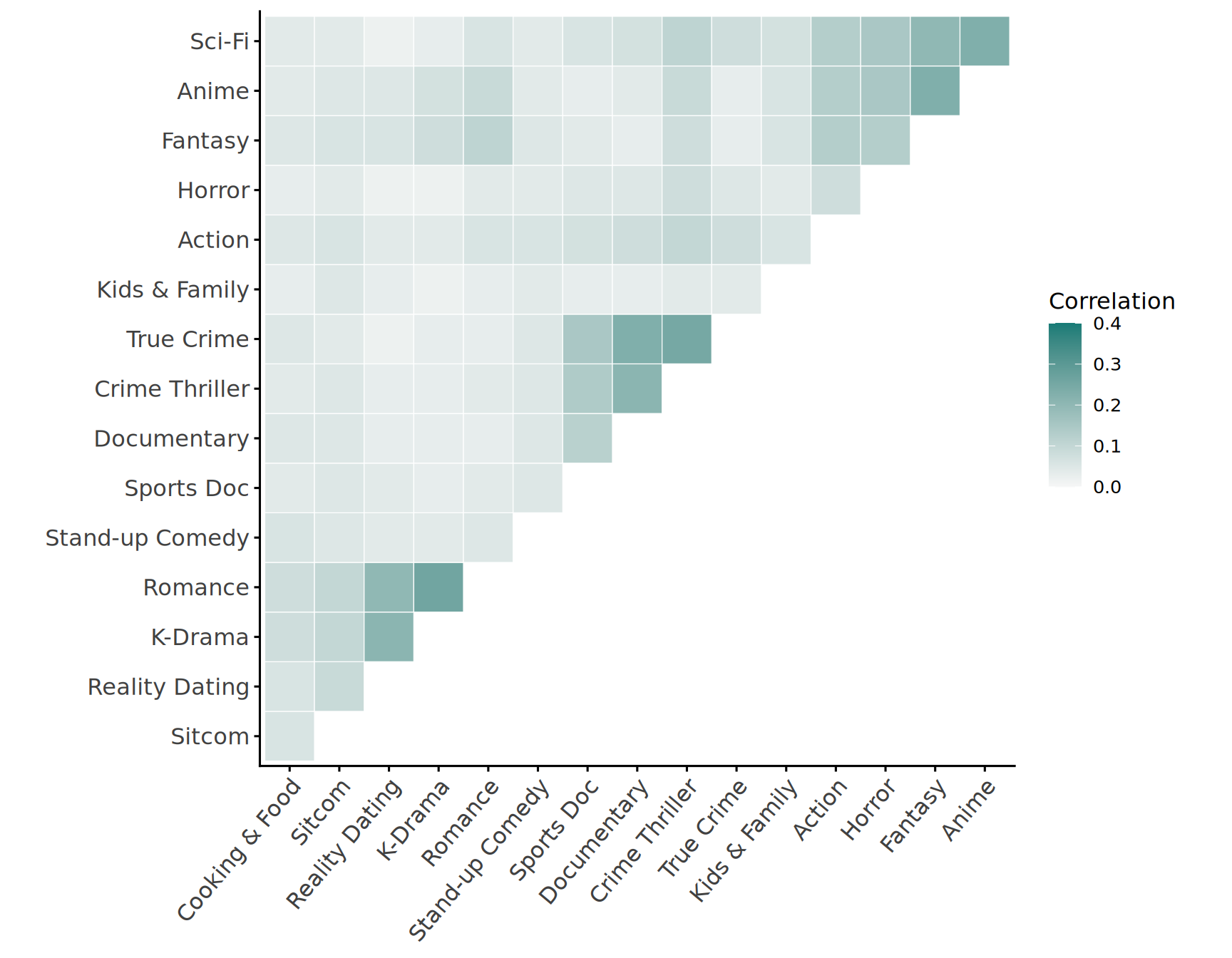
The training data show clusters of correlated genres driven by the same latent factors.
Overestimating the union under independence
A simple approach uses the marginal viewer shares \(\hat p_j\) from the training data and assumes that genre indicators are mutually independent. Under this assumption, the share of users who watched at least one genre in \(S\) is
\[ \hat P_{\mathrm{indep}}\!\left( \bigcup_{j \in S}\{X_j = 1\} \right) = 1 - \prod_{j \in S}(1 - \hat p_j) \]
Genre preferences are not independent, however. Viewers who watch K-Drama are also more likely to watch Romance, so the overlap between the two audiences is larger than independence implies. The independence approximation consequently understates the overlap and overstates the share who watched at least one of the two genres.
Table 1 reports the marginal viewer shares from the training data, the union implied by independence, and the union observed in the validation data.
| K-Drama share | Romance share | Independence estimate | Observed union | Relative overestimate |
|---|---|---|---|---|
| 34.7% | 40.1% | 60.9% | 54.8% | 11.1% |
For a population of 20 million, an error of only a few percentage points in the union probability can translate into an overestimate on the order of a million users.
Approximating the joint distribution with LCA
The independence approximation makes union probabilities easy to calculate but cannot represent co-occurrence across genres. An LCA with \(K\) classes—equivalently, a Bernoulli mixture model—retains the simple probability calculation while allowing for dependence at the population level.
\[ P(\mathbf{x}) = \sum_{k=1}^K\pi_k\prod_{j=1}^J \theta_{jk}^{x_j}(1 - \theta_{jk})^{1-x_j}, \qquad \mathbf{x} \in \{0,1\}^J \]
Here, \(\pi_k\) is the mixing proportion for class \(k\), and \(\theta_{jk}\) is the probability that a viewer in class \(k\) watches genre \(j\). Genre indicators are conditionally independent within each class, but mixing multiple classes induces dependence in the population. I estimate the model with the EM algorithm implemented in {flexmix}.
The model has \(K(J + 1) - 1\) free parameters: more than the 16 parameters in the independence model, but far fewer than the \(2^{16} - 1 = 65{,}535\) required by the saturated model. Setting \(K = 1\) recovers the independence model, while larger values of \(K\) can represent richer dependence structures.
I do not interpret the latent classes themselves. Instead, I use the mixture to approximate \(P(\mathbf{x})\) and evaluate it by the accuracy of UU estimates across genre combinations. Label switching is immaterial because relabeling the classes leaves both the fitted distribution and the resulting UU estimates unchanged.
Computing UU for arbitrary conditions
Conditional on class \(k\), the genre indicators are independent. Let \(A\) be the set of genres required to be present and \(B\) the set required to be absent. Then
\[ P\!\left( \bigcap_{j \in A}\{X_j = 1\}\; \cap \;\bigcap_{j \in B}\{X_j = 0\} \right) = \sum_{k=1}^K\pi_k \prod_{j \in A}\theta_{jk}\prod_{j \in B}(1 - \theta_{jk}) \]
The probability of watching at least one genre in \(S\) is the complement of watching none of them:
\[ P\!\left( \bigcup_{j \in S}\{X_j = 1\} \right) = 1 - \sum_{k=1}^K\pi_k\prod_{j \in S}(1 - \theta_{jk}) \]
This calculation has complexity \(O(K|S|)\) and requires only the fitted parameters. The same model also handles intersections and exclusions, such as “watched Anime but not Horror,” through the corresponding products of \(\theta_{jk}\) and \(1 - \theta_{jk}\).
Selecting the number of classes using validation data
I compare \(K \in \{1,2,3,4,6,8,12,16\}\). Every model is fitted exclusively on the 50,000-viewer training set. The evaluation covers all 120 two-way, 560 three-way, and 1,820 four-way genre unions. For each query, I compare the estimated union probability with its empirical counterpart in the validation data. I exclude one-way queries because their marginal probabilities can be estimated directly from the training data.
Let \(u_q\) denote the union probability observed in the validation data and \(\hat u_{q,K}\) the estimate from the model with \(K\) classes. I select \(K\) using RMSE on the probability scale across all two-way, three-way, and four-way queries. Every combination receives equal weight, so query sizes with more possible combinations contribute more to the overall RMSE. With \(Q\) total queries, the criterion is
\[ \operatorname{RMSE}(K) = \sqrt{\frac{1}{Q}\sum_{q=1}^{Q}(\hat u_{q,K} - u_q)^2} \]
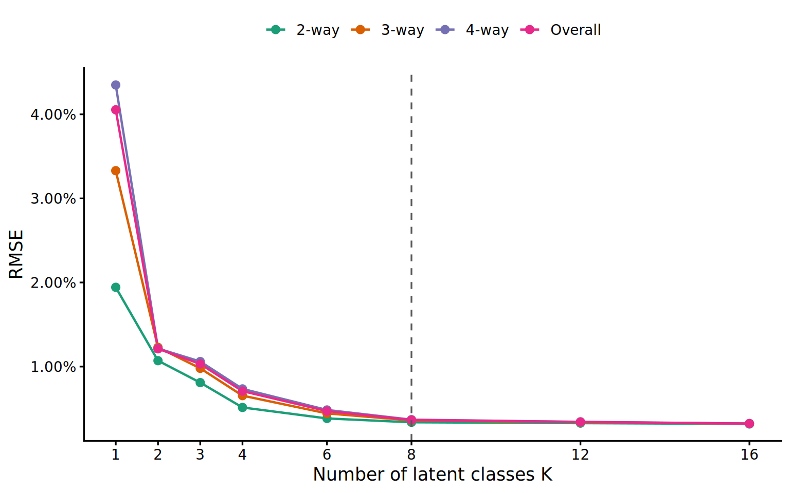
RMSE declines through \(K = 8\) and improves only slightly thereafter. Balancing approximation accuracy against model complexity, I select \(K = 8\).
Approximation accuracy on the test set
After fixing \(K\), I evaluate approximation accuracy on an independently generated test set of two million viewers.
Even with synthetic data, an empirical union probability computed from a finite sample varies slightly from one draw to another. This is Monte Carlo error. Increasing the test set to two million viewers reduces this variation and brings the observed union probabilities close to their population values. The remaining discrepancies therefore reflect model approximation error more than random variation in the test data. The test set is used neither to fit the model nor to select \(K\).
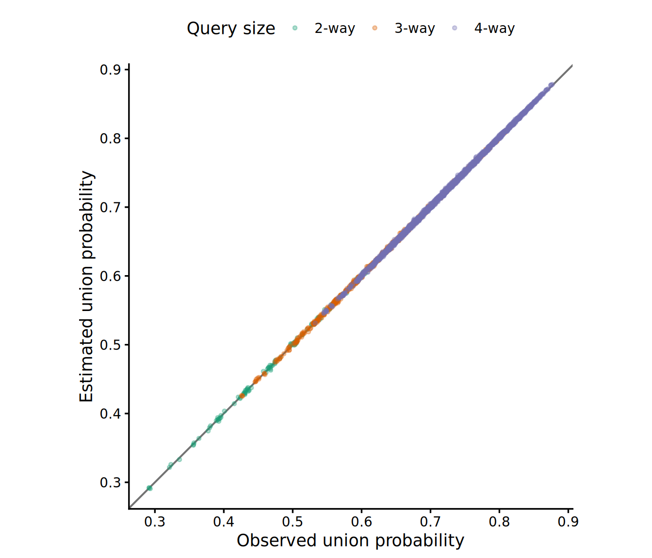
I compare the estimates from the selected LCA with union probabilities observed in the test data. Points closer to the 45-degree line indicate smaller approximation errors.
| Query size | RMSE | Mean relative error | 95th percentile relative error | Maximum relative error |
|---|---|---|---|---|
| 2-way | 0.19% | 0.33% | 0.80% | 1.08% |
| 3-way | 0.19% | 0.25% | 0.58% | 1.01% |
| 4-way | 0.19% | 0.21% | 0.49% | 0.96% |
Summary
Audience sizes cannot generally be added when targeting conditions overlap. Modeling the joint distribution of genre indicators provides a way to account for that overlap while avoiding repeated scans of user-level data.
In this example, I used latent class analysis not to interpret latent audience segments, but as a compact approximation to the joint distribution. The number of classes was selected using validation error on the downstream UU queries rather than an information criterion.
Once fitted, the model can answer arbitrary genre-union queries from the estimated parameters alone. The practical value is therefore less about discovering latent classes and more about turning a large set of overlapping audience definitions into a reusable query layer.
Implementation
Once the model is fitted, the only quantities required for aggregation are the class proportions \(\hat\pi_k\) and the class-specific genre probabilities \(\hat\theta_{jk}\).
library(tidyverse)
library(flexmix)

set.seed(2029)
sf <- stepFlexmix(
  X_train ~ 1,
  k = selected_k,
  nrep = 3,
  model = FLXMCmvbinary(),
  verbose = FALSE
)
fit <- getModel(sf, which = as.character(selected_k))

pi_hat <- prior(fit)
theta_hat <- parameters(fit)

uu_union <- function(pi_hat, theta_hat, S) {
  1 - sum(pi_hat * apply(1 - theta_hat[S, , drop = FALSE], 2, prod))
}

s_pair <- c("K-Drama", "Romance")
S <- match(s_pair, colnames(X_train))
uu_union(pi_hat, theta_hat, S)