In this series, several approaches to estimating the effect are applied to the same dataset. This first article builds that dataset and works through the pre-post comparison that everyone tries first.
Suppose you are a data scientist at a video streaming service that runs on a wide range of devices.
On 2026-06-01, users became able to pause a video ad, but only on iOS devices. Users cannot skip ads while watching. So, before this feature, the only way to stop watching during an ad was to close the app or the browser. In that case, the play was counted as incomplete. This feature is expected to replace some of these exits, so the completion rate on iOS should increase.
After the release, the dashboard shows a higher completion rate on iOS than before. You’d want to report “the feature is working,” but all you have is daily completion rates by device. Data in this format, the same units (devices, in this case) observed repeatedly over time, is called a panel, and I’ll use that term from here on. So, can we look at this panel and say “the feature lifted the completion rate by X points”?
This article does two things:
Pre-post comparison: compute the estimate everyone tries first, and confirm with numbers that it cannot separate an effect from everything else moving at the same time. As we’ll see, running it on a date where nothing was released produces an “effect” of \(+0.62\) percentage points (pp from here on), around 60% of the true effect, and nothing in the data marks it as spurious.
Synthetic data design: build the validation dataset used throughout this series. The series covers difference-in-differences (DiD), the synthetic control method (SCM), CausalImpact, and a randomized comparison, and the backbone of all four is synthetic data whose true treatment effect is known. As long as we know the answer, we can score how far off each method is.
Defining the metrics
An impression is one ad play start, and a complete is a play that ran to the end. The completion rate is defined as \(\text{complete} / \text{impression}\). The table below maps how a play can end to the two metrics; every play that starts counts as exactly one impression, however it ends.
| How the play ends | impression | complete |
|---|---|---|
| Played to the end | 1 | 1 |
| Paused, then resumed and played to the end | 1 | 1 |
| App or browser closed to stop watching (an exit) | 1 | 0 |
| Cut off by a network failure or an app crash | 1 | 0 |
The pause feature can only act on the third row. The mechanism from the opening is exactly this: shift some of those exits into the second row, and the completion rate goes up. It cannot rescue unintentional incomplete plays like the fourth row. This boundary matters later, in the sanity check on the size of the true effect.
One more assumption: whether a play counts as complete is settled within the same day. Pauses are assumed to be short, so a play that starts on day \(t\) is resolved as complete or incomplete within day \(t\).
A pre-post comparison on iOS alone
The simplest way to measure the effect is to compare the completion rates before and after the release. Pick an anchor date \(t_0\) and time window lengths \(k_{\text{pre}}, k_{\text{post}}\), then compute the following difference:
\[ \hat{\Delta}(t_0;\, k_{\text{pre}}, k_{\text{post}}) = \frac{\sum_{t \in W_{\text{post}}} x_t}{\sum_{t \in W_{\text{post}}} n_t} - \frac{\sum_{t \in W_{\text{pre}}} x_t}{\sum_{t \in W_{\text{pre}}} n_t} \]
Here, \(n_t\) and \(x_t\) are the impressions and completes for iOS on day \(t\), with the time windows defined as \(W_{\text{pre}} = [t_0 - k_{\text{pre}},\, t_0)\) and \(W_{\text{post}} = [t_0,\, t_0 + k_{\text{post}})\). Results are reported in pp.
For comparison, prepare a fake anchor date as well: run the same calculation on a date with no release anywhere near it, and watch how the estimator behaves where the true answer is zero. This is the same idea as a placebo in drug trials, hence the name: the placebo anchor date. The date is 2026-03-02, a Monday, matching the day of the week of the actual release. It also splits the pre-period in half, so a 91-day window on each side of it covers the pre-period exactly.
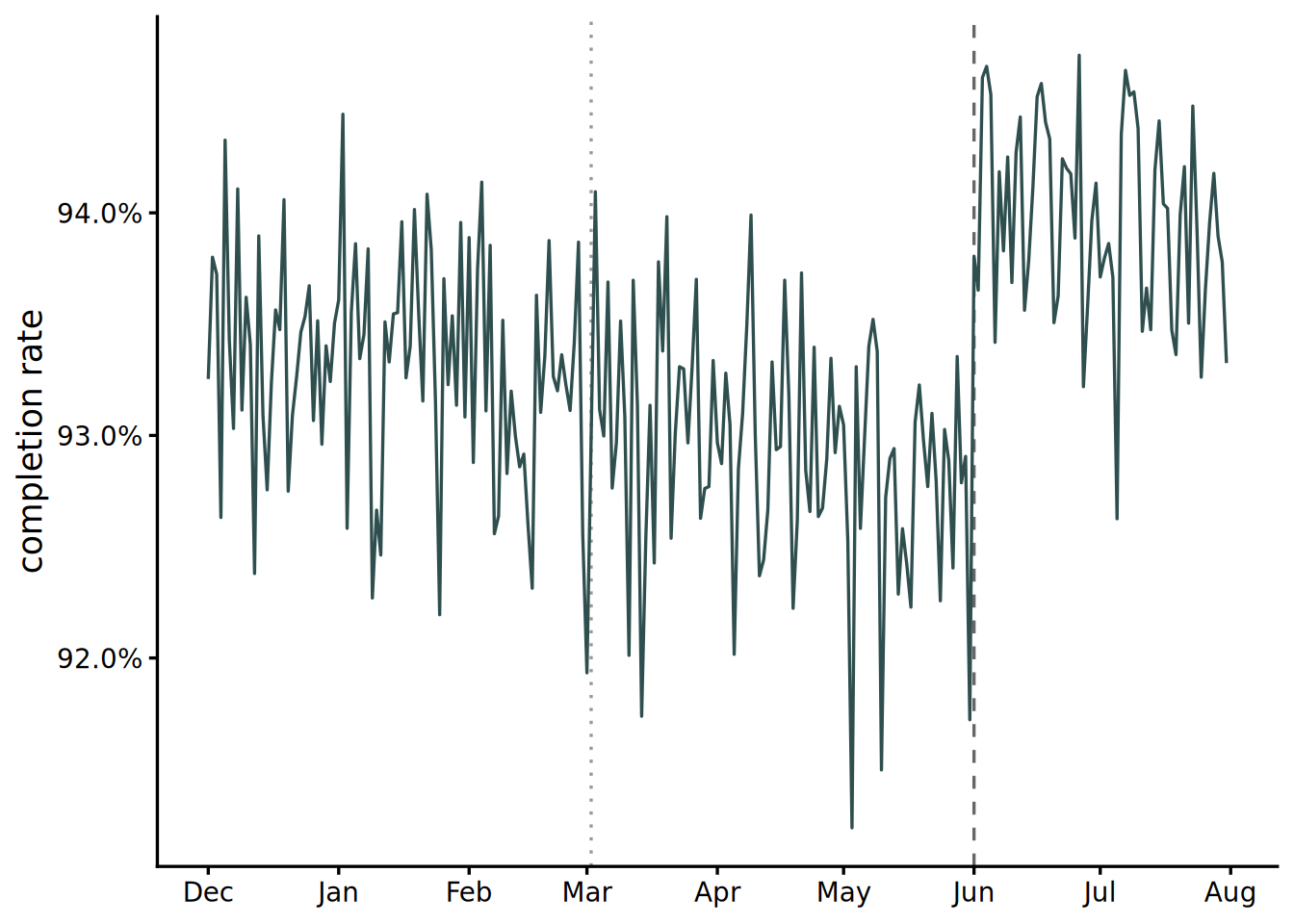
Figure 1 shows three movements mixed together in the series: a weekly cycle that dips 0.4 to 0.6pp on weekends, a slow trend that drifts down by about 0.6pp over the eight months, and daily noise with a standard deviation of around 0.4pp. A pre-post difference picks up all three, with no way to tell them apart from the treatment effect.
Table 1 shows how much gets picked up: four time windows anchored at the release date, and four more at the placebo anchor date 13 weeks earlier, eight estimates in total. The three shorter windows are the same on both sides. The longest one differs, because each anchor has a different amount of data around it: 182 days before and 61 days after the release, and 91 days on each side of the placebo anchor.
| Anchor | Pre (days) | Post (days) | Estimate (pp) |
|---|---|---|---|
| release 2026-06-01 | 182 | 61 | +0.85 |
| release 2026-06-01 | 28 | 28 | +1.28 |
| release 2026-06-01 | 7 | 7 | +1.41 |
| release 2026-06-01 | 3 | 3 | +1.57 |
| placebo 2026-03-02 | 91 | 91 | −0.38 |
| placebo 2026-03-02 | 28 | 28 | −0.05 |
| placebo 2026-03-02 | 7 | 7 | +0.17 |
| placebo 2026-03-02 | 3 | 3 | +0.62 |
Start with the placebo side, where the right answer is zero. The estimates run from \(-0.38\) to \(+0.62\)pp, and the \(+0.62\)pp is around 60% of the true effect on the release side. A feature that was never shipped produces a number a reviewer would accept as a result. On the release side, the estimate runs from \(+0.85\)pp with the longest window to \(+1.57\)pp with the 3-day window, so the choice of window alone moves the answer by \(0.7\)pp. Both sides come out of the same estimator, and nothing in the output distinguishes them.
The mechanism is exactly the structure visible in the figure. A short, asymmetric window like the 3-day one imports the weekly cycle: with a Monday anchor, the three days before are Friday through Sunday and the three days after are Monday through Wednesday, so the weekend dip turns straight into the difference. A long window imports the trend instead: with 182 days before the release and 61 days after it, the center of the pre-period sits about four months before the center of the post-period, so four months of slow decline accumulate in the difference. And in both cases, sampling noise rides on top.
The key point is that there is no way to separate these three components from the treatment effect using this series alone. The question a pre-post comparison answers is “did the completion rate change over time,” and the feature is only one of the things that changed during that time. A pre-post comparison on observational data is not a stand-in for the counterfactual.
Designing the synthetic data
So, can DiD separate them? What about SCM, or CausalImpact? Working through that question one method at a time is what this series is for, and checking an answer requires a scoring key: the right answer. That is why the panel shown so far is synthetic.
Two simplifications. First, the effect is constant from the day of release; no gradual adoption ramp is modeled. Second, the treatment does not affect the number of impressions. Preventing an exit could in reality extend the session and add exposure, but generating the denominator independently of the treatment does not affect a rate analysis, so that path is cut here.
Design requirements
The true treatment effect is known. Every estimator in this series is checked against it, and the first to be scored is the set of eight pre-post estimates above.
Devices differ in level while sharing the weekly cycle and the slow trend. This is exactly the confounding structure that broke the pre-post comparison, and at the same time the structure that comparison-based methods rely on.
The iOS level sits inside the convex hull of the control devices, that is, between the minimum and the maximum of the controls. Why this matters is explained in the third article (SCM); here it is only stated as a requirement.
The generating model
The panel is generated directly as device-by-day aggregate cells; no individual users are created. Users exist only as a per-device volume scale \(M_d\).
\[ n_{dt} \sim \text{Poisson}(1.5\, M_d), \qquad x_{dt} \sim \text{Binomial}(n_{dt},\, p_{dt}) \]
\[ \text{logit}\, p_{dt} = \alpha_d + w_{\text{dow}(t)} + \gamma \cdot \frac{t}{T_{\text{total}}} + \tau \cdot 1\{d = \text{ios},\ t \geq T\} \]
\(n_{dt}\) is the number of impressions for device \(d\) on day \(t\), \(x_{dt}\) is the number of completes, and \(p_{dt}\) is the probability that one impression ends as a complete. What happens here is addition on the logit scale: a device-specific intercept \(\alpha_d\), plus the day-of-week effect \(w\), plus a slow trend \(\gamma\) shared by all devices, plus the treatment effect \(\tau\) that applies only to iOS after the release. \(t / T_{\text{total}}\) is the elapsed fraction of the full period and runs from 0 to 1. The period runs from 2025-12-01 to 2026-07-31, 243 days in total, with the release at \(T =\) 2026-06-01, splitting it into 182 pre-period days and 61 post-period days.
Parameters
| Device | Role | \(p\) at \(t = 0\) | \(\alpha_d\) | \(M_d\) |
|---|---|---|---|---|
| ios | treated | 93.5% | 2.67 | 2,700 |
| android | control | 92.5% | 2.51 | 1,300 |
| pc-web | control | 92.5% | 2.51 | 800 |
| android-tv | control | 96.5% | 3.32 | 800 |
| smart-tv-a | control | 95.5% | 3.06 | 800 |
| smart-tv-b | control | 92.0% | 2.44 | 800 |
| smart-tv-c | control | 97.0% | 3.48 | 500 |
| tv-web | control | 96.0% | 3.18 | 500 |
| mobile-web | control | 94.5% | 2.84 | 500 |
| streaming-stick | control | 97.2% | 3.55 | 300 |
| game-console | control | 95.0% | 2.94 | 300 |
Table 2 lists the values that differ by device; the remaining parameters are common to all of them. The day-of-week effect is \(0\) for Monday through Thursday, \(+0.02\) for Friday, \(-0.06\) for Saturday, and \(-0.09\) for Sunday, the common trend is \(\gamma = -0.10\) over the full period, and the treatment effect is \(\tau = +0.17\), all on the logit scale. The random seed is fixed at 1. Converted to the iOS level, these give a weekend dip of 0.4 to 0.6pp, a decline of \(-0.63\)pp from the trend over the full period, and binomial noise of about 0.4pp in standard error at roughly 4,000 impressions per day. The three movements visible in the first figure correspond, in order, to the day-of-week effect, the common trend, and the draw from the binomial distribution.
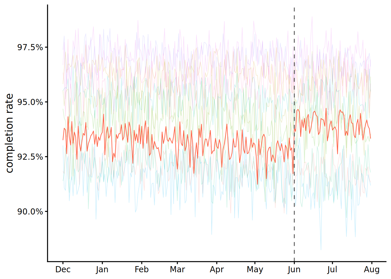
Figure 2 shows requirements 2 and 3 realized. All 11 series share the same weekend dip and the same downward trend; what differs is the level and the coarseness of the noise, which follows how small \(M_d\) is. The iOS pre-period level is 93.1%, fourth lowest of the 11 devices, sitting neatly inside the control range of 91.5 to 97.1%.
The true treatment effect
The true value used here is the average treatment effect on the treated (ATT), on the pp scale. Concretely, for each iOS post-period cell, take the difference between the generating rate with \(\tau\) and the generating rate without it, then average those differences weighted by impressions.
\[ \text{ATT} = \frac{\sum_{t \geq T} n_{\text{ios},t} \left[ \sigma(\ell_{\text{ios},t}) - \sigma(\ell_{\text{ios},t} - \tau) \right]}{\sum_{t \geq T} n_{\text{ios},t}} = +1.049 \text{ pp} \]
\(\sigma\) is the logistic function and \(\ell\) the linear predictor including the treatment. This value comes from the generating equation, not from an estimate based on the realized completes. The only part the seed touches is the weight \(n\) drawn from the Poisson, so it works as a fixed yardstick in practice. From here on, every estimator in this series is reported next to this \(+1.049\)pp.
The size of the effect deserves a sanity check against the mechanism. Without treatment, the iOS completion rate on a weekday at the start of the period is \(\sigma(2.67) = 93.5\%\), which means 6.5pp of plays end incomplete. A true effect of \(+1.05\)pp converts one sixth of that into completes. Incomplete plays also include network failures and crashes, so among deliberate exits alone, the share the pause feature takes over is larger than one sixth. That is an aggressive number for a single feature, but the order of magnitude is realistic, and it is nowhere near a fantasy value that would eat up the entire pool of incomplete plays.
Two variants from one random stream
The generator outputs two datasets: parallel, the main line, and divergent, in which iOS alone drifts away from the pre-period onward. The divergent variant adds \(\delta \cdot t / T_{\text{total}}\) (\(\delta = +0.30\)) to the iOS logit, opening a gap of about 1.3pp by the end of the pre-period. In the second article, this variant plays the world where the assumption behind the method breaks.
The trick is in qbinom. qbinom(r, n, p) passes a uniform draw \(r\) through the binomial quantile function; the distribution is the same as rbinom(1, n, p), but the result is determined once \(r\) is fixed. A single \(r\) per cell is shared by both variants, so control cells, where both \(n\) and \(p\) are identical, produce bit-identical completes (verified: all(complete_parallel == complete_divergent) returns TRUE for the control devices). The iOS cells have different \(p\) across variants, so their values do not match, but they pass through the same \(r\) and their noise moves in the same direction (comonotone). If an analysis of the two files differs, then, the difference comes from the divergent trend term, not from a fresh draw of the random numbers.
The output files are panel_parallel.csv and panel_divergent.csv, both with the schema date, device, post, impression, complete, complete_rate. post can be derived from the release date, but it is kept as a column for convenience.
Decomposing the comparison with the true values
Requirement 1 pays off right here. With synthetic data, both the treated generating rate \(p_{dt} = \sigma(\ell_{dt})\) and the untreated one \(p^0_{dt} = \sigma(\ell_{dt} - \tau \cdot 1\{d = \text{ios},\ t \geq T\})\) are available for every cell. Replacing the completes inside \(\hat{\Delta}\) with these rates gives the expectation conditional on the impression counts, and that expectation splits exactly into a treatment component and a contamination component.
\[ \hat{\Delta} = \underbrace{\left[ m(W_{\text{post}}) - m(W_{\text{pre}}) \right] - \left[ m^0(W_{\text{post}}) - m^0(W_{\text{pre}}) \right]}_{\text{treatment}} + \underbrace{m^0(W_{\text{post}}) - m^0(W_{\text{pre}})}_{\text{contamination}} + \text{noise} \]
Here \(m(W) = \sum_{t \in W} n_t p_t / \sum_{t \in W} n_t\), and \(m^0\) is the same quantity computed with \(p^0\). The contamination term is the pre-post difference in a world where \(\tau = 0\); the influence of the trend and of the day-of-week composition of the window collects here. The noise is the residual, the realized value minus its expectation.
| Anchor | Pre (days) | Post (days) | Estimate | Treatment | Contamination | Noise |
|---|---|---|---|---|---|---|
| release 2026-06-01 | 182 | 61 | +0.85 | +1.05 | −0.31 | +0.11 |
| release 2026-06-01 | 28 | 28 | +1.28 | +1.04 | −0.08 | +0.31 |
| release 2026-06-01 | 7 | 7 | +1.41 | +1.04 | −0.02 | +0.38 |
| release 2026-06-01 | 3 | 3 | +1.57 | +1.02 | +0.29 | +0.26 |
| placebo 2026-03-02 | 91 | 91 | −0.38 | 0.00 | −0.24 | −0.14 |
| placebo 2026-03-02 | 28 | 28 | −0.05 | 0.00 | −0.07 | +0.02 |
| placebo 2026-03-02 | 7 | 7 | +0.17 | 0.00 | −0.02 | +0.19 |
| placebo 2026-03-02 | 3 | 3 | +0.62 | 0.00 | +0.28 | +0.35 |
Table 3 is the reveal behind Table 1. The treatment component barely moves across the four release-side windows, staying between \(+1.02\) and \(+1.05\)pp; what looked like movement was contamination and noise all along.
Contamination changes sign with the window. For the longest release-side window it is \(-0.31\)pp, and the cause is the trend: the centers of the pre-period and the post-period are 0.50 apart in elapsed fraction \(t/T_{\text{total}}\), about four months in days, and a logit decline of \(-0.10 \times 0.50 = -0.050\) works out to \(-0.31\)pp at the iOS level. For the 3-day window it is \(+0.29\)pp, and the cause is the day-of-week composition: the pre side is Friday through Sunday (average \(w\) of \(-0.043\)) and the post side is Monday through Wednesday (\(w = 0\)), so that gap carries straight through. The 7-day and 28-day windows are balanced across days of the week and too short for the trend to bite, so contamination is nearly zero; noise of \(+0.31\) to \(+0.38\)pp takes over as the main source of error instead.
In real data, only the first numeric column of this table is observable. On a real panel there is no way to split the \(+1.41\)pp from the 7-day window into “\(+1.04\) of effect and \(+0.38\) of luck.” That single point is the reason this series runs on synthetic data. In the articles that follow, each estimate is reported next to the true value of \(+1.049\)pp, and the gap between them is settled by attribution rather than argument.
R code
The generator below is the canonical implementation for this series. Running it writes the two CSV files that every later article reads, so the next article on DiD starts from data/panel_parallel.csv rather than regenerating the panel.
library(tidyverse)

devices <- tribble(
  ~device           , ~treated , ~alpha , ~m_users ,
  "ios"             , TRUE     , 2.67   ,     2700 ,
  "android"         , FALSE    , 2.51   ,     1300 ,
  "pc-web"          , FALSE    , 2.51   ,      800 ,
  "android-tv"      , FALSE    , 3.32   ,      800 ,
  "smart-tv-a"      , FALSE    , 3.06   ,      800 ,
  "smart-tv-b"      , FALSE    , 2.44   ,      800 ,
  "smart-tv-c"      , FALSE    , 3.48   ,      500 ,
  "tv-web"          , FALSE    , 3.18   ,      500 ,
  "mobile-web"      , FALSE    , 2.84   ,      500 ,
  "streaming-stick" , FALSE    , 3.55   ,      300 ,
  "game-console"    , FALSE    , 2.94   ,      300
)

w_dow <- tribble(
  ~wday , ~w    ,
      1 ,  0    , # Mon
      2 ,  0    , # Tue
      3 ,  0    , # Wed
      4 ,  0    , # Thu
      5 ,  0.02 , # Fri
      6 , -0.06 , # Sat
      7 , -0.09 # Sun
)

# logit-scale components (gamma, tau, delta in the article notation)
trend_common <- -0.10 # common trend over the full period
effect_treatment <- 0.17 # treatment effect on ios
trend_divergence <- 0.30 # ios-specific trend, divergent variant only
imp_per_user_day <- 1.5 # expected impressions per user-day
date_treat <- lubridate::ymd("2026-06-01")

days <- tibble(
  date = seq(
    lubridate::ymd("2025-12-01"),
    lubridate::ymd("2026-07-31"),
    by = "day"
  )
) |>
  mutate(
    wday = lubridate::wday(date, week_start = 1),
    post = date >= date_treat,
    t_frac = (row_number() - 1) / (n() - 1)
  ) |>
  inner_join(w_dow, by = "wday") |>
  arrange(date)

# inverse transform sampling: qbinom(r, n, p) is deterministic given r,
# so both variants share randomness and control units coincide exactly

set.seed(1)

panel_gen <- crossing(devices, days) |>
  mutate(
    impression = rpois(n(), imp_per_user_day * m_users),
    r = runif(n()),
    logit_parallel = alpha +
      w +
      trend_common * t_frac +
      effect_treatment * post * treated,
    logit_divergent = logit_parallel + trend_divergence * t_frac * treated,
    complete_parallel = qbinom(r, impression, plogis(logit_parallel)),
    complete_divergent = qbinom(r, impression, plogis(logit_divergent))
  )

panel <- panel_gen |>
  pivot_longer(
    c(complete_parallel, complete_divergent),
    names_to = "variant",
    names_prefix = "complete_",
    values_to = "complete"
  ) |>
  mutate(complete_rate = complete / impression) |>
  select(variant, date, device, post, impression, complete, complete_rate)

# ATT: derived from the generating equation, not estimated from the completes
panel_gen |>
  filter(treated, post) |>
  summarise(
    att = weighted.mean(
      plogis(logit_parallel) - plogis(logit_parallel - effect_treatment),
      impression
    )
  )
#> # A tibble: 1 x 1
#>      att
#>    <dbl>
#> 1 0.0105

# structural check: control units identical across variants, by construction
panel_gen |>
  filter(!treated) |>
  summarise(identical = all(complete_parallel == complete_divergent))
#> # A tibble: 1 x 1
#>   identical
#>   <lgl>
#> 1 TRUE

dir.create("data", showWarnings = FALSE)

panel |>
  filter(variant == "parallel") |>
  select(-variant) |>
  write_csv("data/panel_parallel.csv")

panel |>
  filter(variant == "divergent") |>
  select(-variant) |>
  write_csv("data/panel_divergent.csv")
Each file has 2,673 rows, 11 devices over 243 days, with the schema date, device, post, impression, complete, complete_rate. The variant column is dropped on the way out, so the two files are interchangeable as inputs: an analysis written against one runs unchanged against the other.