The previous article set up a scenario in which an AVOD service released an ad pause feature on 2026-06-01, on iOS only, and generated a panel of daily ad completion rates for all 11 devices. The true effect of the feature was set to +1.049 percentage points (pp from here on) as the ATT (average treatment effect on the treated).
A simple pre-post comparison on this data failed to recover the true value. A date with no release produced an “effect” of +0.62pp, suggesting that the day-of-week cycle, the trend, and noise had leaked into the difference. One reason pre-post comparisons fail is exactly this contamination by time variation other than the treatment.
What if there were data from another device exposed to the same time variation? Subtracting that device’s pre-post difference from the iOS one should cancel just the contamination. This is the idea behind the well-known difference-in-differences (DiD) approach. So this time, the true causal effect is estimated with DiD.
This article does the following three things:
- Define the DiD estimator, and lay out the condition for the cancellation to work (the parallel trends assumption) and the conditions a group must satisfy to serve as the control.
- Run a visual inspection and a slope test on the gap over the pre-period series of the treated and control groups, checking that the trends are parallel.
- Apply the same 7-day-window DiD to a dataset where parallel trends hold and to one where they do not, and confirm numerically that the former’s CI covers the true value while the latter’s excludes it.
The DiD estimator
The treated group is fixed to iOS, and the device used as the control is denoted \(c\). For device \(d\) and period \(W \in \{\text{pre}, \text{post}\}\), define the completion rate as \(\bar{Y}_{d,W} = \sum_{t \in W} x_{dt} \big / \sum_{t \in W} n_{dt}\), where \(n\) is the number of impressions and \(x\) the number of completes. The DiD estimator is the difference of the pre-post differences.
\[ \hat{\tau}_{\text{DiD}} = \left( \bar{Y}_{\text{iOS},\text{post}} - \bar{Y}_{\text{iOS},\text{pre}} \right) - \left( \bar{Y}_{c,\text{post}} - \bar{Y}_{c,\text{pre}} \right) \]
When the expectation of \(\bar{Y}_{d,W}\) has an additive structure in a device level \(\mu_d\), a time effect \(\lambda_W\), and a treatment effect \(\tau\), the terms that the subtractions cancel are as follows.
| pre | post | Post − pre | |
|---|---|---|---|
| iOS | \(\mu_{\text{iOS}} + \lambda_{\text{pre}}\) | \(\mu_{\text{iOS}} + \lambda_{\text{post}} + \tau\) | \((\lambda_{\text{post}} - \lambda_{\text{pre}}) + \tau\) |
| Control \(c\) | \(\mu_c + \lambda_{\text{pre}}\) | \(\mu_c + \lambda_{\text{post}}\) | \(\lambda_{\text{post}} - \lambda_{\text{pre}}\) |
| DiD | \(\tau\) |
The difference along each row cancels \(\mu_d\), and the difference between the rows cancels \(\lambda_W\). The day-of-week cycle and the trend that broke the pre-post comparison both belong to \(\lambda_W\), so they cancel whenever this structure holds. This table, however, rests on the following two conditions.
The parallel trends assumption
The time effect must be common across devices. \(\lambda_W\) contains not only trends but also transient fluctuations, so what textbooks call the common shocks assumption is folded in here. Written in counterfactual terms,
\[ \mathbb{E}\left[ \bar{Y}^0_{\text{iOS},\text{post}} - \bar{Y}^0_{\text{iOS},\text{pre}} \right] = \mathbb{E}\left[ \bar{Y}_{c,\text{post}} - \bar{Y}_{c,\text{pre}} \right] \]
where \(\bar{Y}^0\) is the value in the world without the treatment. The post term on the left-hand side is a counterfactual that cannot be observed in the world where the treatment actually happened, so this equality cannot be tested directly from the data. Its plausibility can be checked from the pre-period behavior, but proving that it holds is impossible in principle.
Conditions on the control group
Obvious as it sounds, the control must be untreated and free of spillover from the treatment. If the treatment effect leaks into the control-side difference, the subtraction shaves exactly that much off \(\hat{\tau}_{\text{DiD}}\).
Why Android as the control
There are 10 candidate devices for the control \(c\); this article uses Android. The reasons are threefold:
- It meets the conditions on the control group. The treatment is a UI change inside the iOS app, and a path by which it spills across devices into the Android completion rate is hard to imagine.
- Its confounding structure is the closest. As the same mobile app, its user base and viewing context are the closest to iOS, and among the candidates it is the most likely to share the time effect.
- It has the largest daily impression volume among the candidates, which keeps the control-side noise the smallest.
All three, however, rest on the analyst’s prior knowledge, with no backing from the data.
The analysis windows
The analysis uses all 182 days of data before the release (the pre window) and the 7 days from the release date (the post window).
The post window is 7 days because that is the shortest length in which the days of the week complete one full cycle. If the pre and post windows each contain every day of the week in equal proportion, the day-of-week effect drops out the moment the pre-post difference is taken. Both windows here contain every day of the week in equal proportion, so this contamination does not occur. A day-of-week-balanced window could also be 14 or 28 days; here the shortest, 7 days, is used.
Using the entire pre-period, in turn, is possible because the situation differs from the pre-post comparison. There, a long window pulled in the trend. In DiD, the common trend enters the control-side difference by the same amount and cancels, under parallel trends, the moment the difference is taken. Taking a long pre-period therefore has no downside; if anything it is a bargain, since the noise shrinks.
Checking parallel trends
The assumption itself cannot be verified, but both devices are observed during the pre-period, so “were they parallel at least in the pre-period?” can be inspected. This is done in two stages: visual inspection and a slope test.
Here the second dataset generated last time comes into play. parallel is the main world where parallel trends hold; divergent is the world where a trend proportional to elapsed time (\(\delta = +0.30\)) is added to the iOS logit only. By the end of the pre-period, a divergence of about 1.3pp has accumulated.
Visual inspection
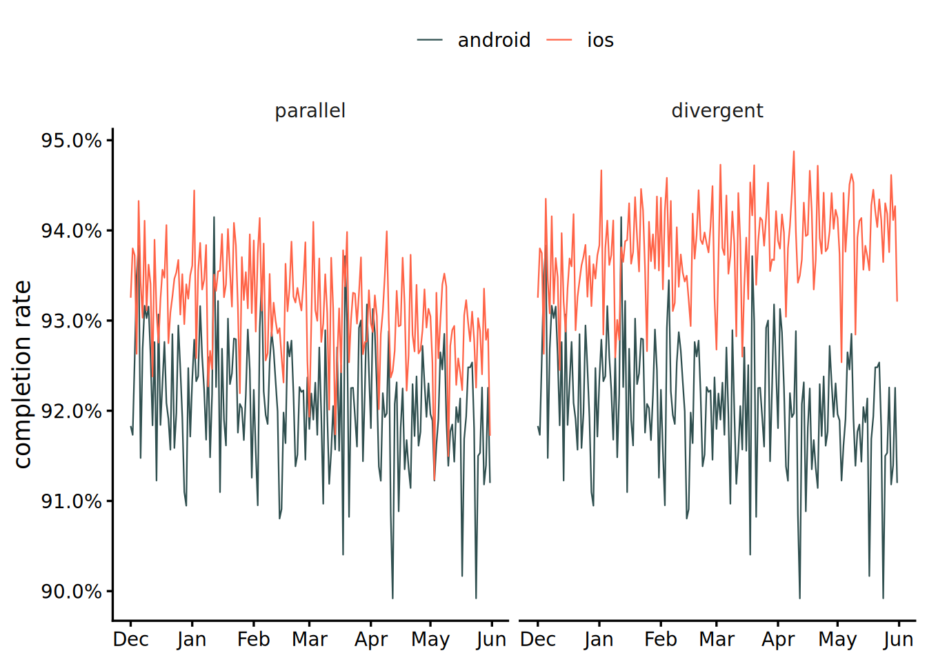
Figure 1 overlays iOS and Android during the pre-period, with parallel on the left and divergent on the right. Even in parallel, where the trends are truly parallel, the two series cross constantly, and whether the parallel trends assumption holds is hard to call.
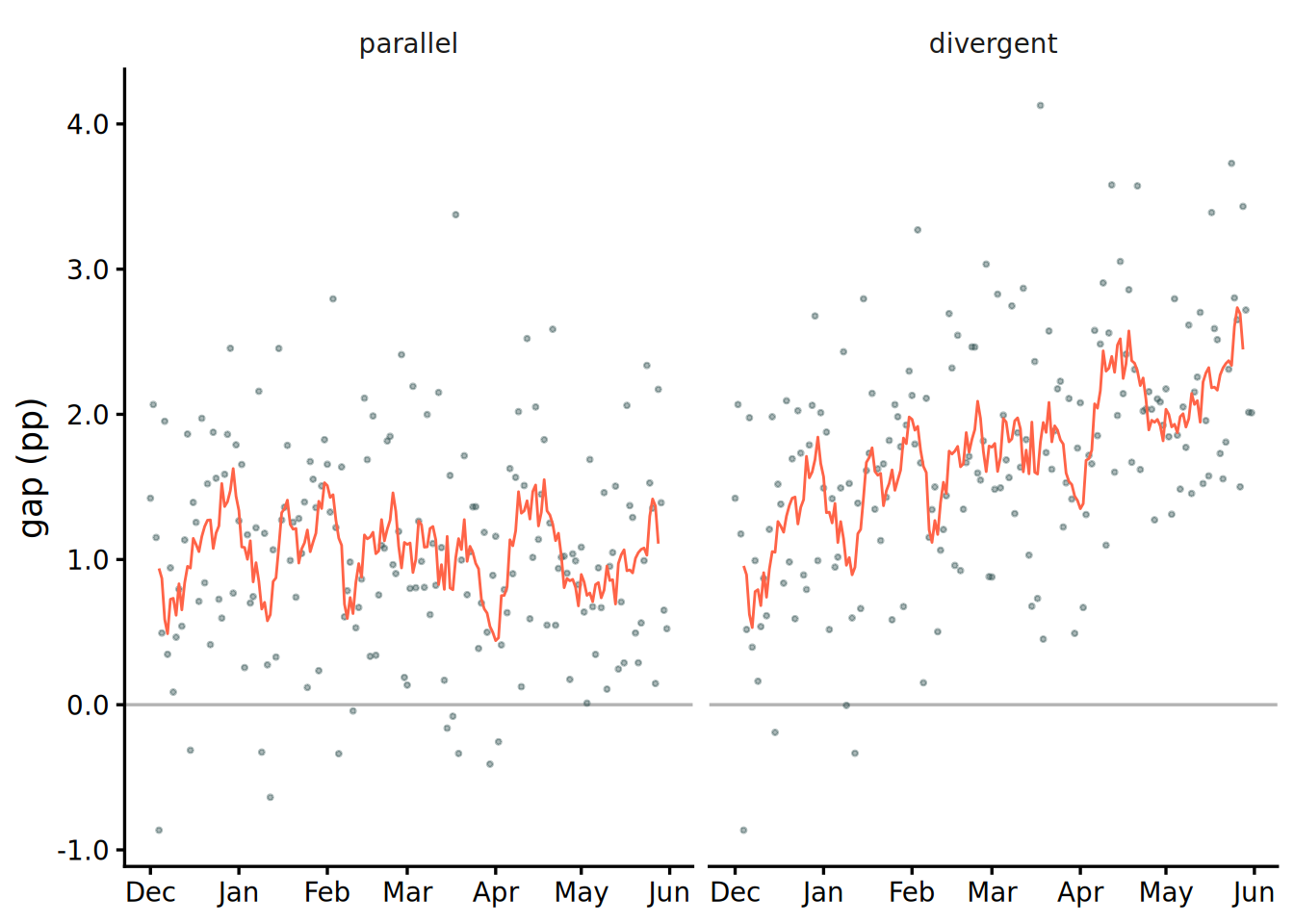
So the noise and the day-of-week cycle are removed before looking again. Figure 2 shows the daily gap \(D_t = Y_{\text{iOS},t} - Y_{\text{And},t}\) and its 7-day moving average. A window of 7 days, the same length as the weekly cycle, wipes out the periodic component and damps the noise. At this point the difference between the two worlds becomes visible: the parallel gap is nearly flat, while the divergent gap climbs.
Slope test on the gap
For a quantitative call, fit a line to the daily pre-period gap \(D_t\) and test whether its slope is zero. The horizontal axis is not raw elapsed days but \(t / T_{\text{pre}}\), scaled to run from 0 at the start of the pre-period to 1 at its end. The slope \(\beta\) can then be read as the gap opened over the entire pre-period.
\[ D_t = \alpha + \beta \cdot \frac{t}{T_{\text{pre}}} + \varepsilon_t, \qquad H_0: \beta = 0 \]
| Characteristic |
parallel
|
divergent
|
||||
|---|---|---|---|---|---|---|
| Beta | 95% CI | p-value | Beta | 95% CI | p-value | |
| Slope (pp) | -0.08 | -0.43, 0.28 | 0.7 | 1.28 | 0.93, 1.64 | <0.001 |
| Abbreviation: CI = Confidence Interval | ||||||
For parallel, \(\hat{\beta} = -0.08\)pp (\(p = 0.68\)): no evidence of divergence. For divergent, \(\hat{\beta} = +1.29\)pp (\(p = 2.1 \times 10^{-11}\)): the null hypothesis is rejected. The divergent point estimate recovers almost exactly the roughly 1.3pp divergence built into the generator, and the slope test cleanly separates the two worlds that visual inspection could not tell apart.
The test’s coverage is limited, though. It sees only linear divergence within the pre-period, so divergence that starts just before the post-period, or nonlinear divergence, never shows up in this regression. And what is actually needed is parallelism in the post-period, which involves the counterfactual and thus cannot be verified in principle.
Estimation
The 7-day-window DiD is applied to both worlds. Each of the four completion rates \(\bar{Y}_{d,W}\) in the estimator is treated as an independent binomial proportion, and the standard error is the square root of the sum of their variances \(\hat{p}_{d,W}(1 - \hat{p}_{d,W}) / n_{d,W}\), where \(n_{d,W}\) is the total number of impressions in the window. This treatment is exact for this data, whose generating process is daily independent binomial draws, but calls for caution on real data: the same users recurring day after day induce autocorrelation, and the standard error tends to be underestimated.
| World | Estimate (pp) | SE (pp) | CI lower (pp) | CI upper (pp) | Truth (+1.049pp) |
|---|---|---|---|---|---|
| parallel | +1.31 | 0.28 | +0.76 | +1.85 | Covered |
| divergent | +1.79 | 0.27 | +1.26 | +2.33 | Excluded |
The parallel estimate is \(+1.31\)pp with a 95% CI of \([+0.76,+1.85]\). The CI excludes 0, so the effect is significant one week after the release, and it covers the true value of \(+1.049\)pp. The \(+0.26\)pp overshoot of the point estimate is \(0.9 \sigma\) against the SE of \(0.28\)pp, within the range of noise. The divergent estimate, in contrast, is \(+1.79\)pp with a 95% CI of \([+1.26,+2.33]\), which does not contain the true value.
Had parallel trends been judged from the raw-series plot alone, skipping the moving average and the slope test, the likely outcome is a confident report of \(+1.79\)pp on divergent as well.
The regression form
The same estimator can be written as a regression. With a treatment dummy \(D = 1\{d = \text{iOS}\}\) and a post dummy \(P = 1\{t \geq T\}\), fit the following model with the daily completion rate as the outcome and the impression count as the weight.
\[ Y_{dt} = \beta_0 + \beta_1 D + \beta_2 P + \beta_3 DP + \varepsilon_{dt} \]
Because this is a saturated model with just the two dummies and their product, \(\hat{\beta}_3\) is algebraically identical to \(\hat{\tau}_{\text{DiD}}\). Indeed, the interaction coefficient from lm(complete_rate ~ treated * post, weights = impression) returns the \(+1.31\)pp of the previous section. In the literature and in practical tooling this is the standard form: adding covariates, generalizing to many groups and periods (two-way fixed effects), and adjusting standard errors all ride on this framework directly.
Computing the standard error takes care. In a panel, the errors of the same device correlate across days, so the default lm standard error tends to be an underestimate. The standard remedy is a cluster-robust standard error clustered by device, but its validity is weak when clusters are few, and it is hard to apply to a 2-unit DiD. A different approach is needed, one that uses the serial-correlation structure or individual-level data.
Arbitrariness in the choice of control
Finally, a problem that remains in this article’s DiD. Android was chosen as the control for three reasons: the conditions on the control group, the closeness of the confounding structure, and volume. All three, though, are the analyst’s qualitative judgments, with no backing from the data. There are 10 candidate devices: pick pc-web and the estimate changes; average all 10 with equal weights and it changes again. If picking one is arbitrary and equal weighting is arbitrary too, the remaining path is to let the data determine the control weights, with the reproduction of the pre-period as the criterion. That is the synthetic control method (SCM), the subject of the next article.
R code
The analysis uses panel_parallel.csv and panel_divergent.csv, generated in the previous article.
library(tidyverse)

date_treat <- lubridate::ymd("2026-06-01")
att_true <- 0.01049 # true ATT

panel <- bind_rows(
  parallel = read_csv("panel_parallel.csv"),
  divergent = read_csv("panel_divergent.csv"),
  .id = "variant"
)

# slope test on the pre-period gap (iOS − Android)
panel |>
  filter(device %in% c("ios", "android"), !post) |>
  pivot_wider(
    names_from = device,
    values_from = complete_rate,
    id_cols = c(variant, date)
  ) |>
  mutate(
    gap = ios - android,
    t_frac = as.integer(date - min(date)) / as.integer(max(date) - min(date)),
    .by = variant
  ) |>
  reframe(
    broom::tidy(lm(gap ~ t_frac, data = pick(everything()))),
    .by = variant
  ) |>
  filter(term == "t_frac") |>
  select(variant, estimate, p.value)
#> variant     estimate   p.value
#> parallel   -0.000806   0.68
#> divergent   0.0129     2.1e-11

# DiD (7-day window, CI from binomial variances)
panel |>
  mutate(k_post = 7) |>
  filter(
    date < date_treat + k_post,
    device %in% c("ios", "android")
  ) |>
  mutate(period = if_else(post, "post", "pre")) |>
  summarise(
    complete = sum(complete),
    impression = sum(impression),
    .by = c(k_post, variant, device, period)
  ) |>
  mutate(
    rate = complete / impression,
    var_rate = rate * (1 - rate) / impression
  ) |>
  pivot_wider(
    names_from = period,
    values_from = c(rate, var_rate),
    id_cols = c(k_post, variant, device)
  ) |>
  mutate(
    diff = rate_post - rate_pre,
    var_diff = var_rate_post + var_rate_pre
  ) |>
  pivot_wider(
    names_from = device,
    values_from = c(diff, var_diff),
    id_cols = c(k_post, variant)
  ) |>
  mutate(
    estimate = diff_ios - diff_android,
    se = sqrt(var_diff_ios + var_diff_android),
    ci_lower = estimate - qnorm(0.975) * se,
    ci_upper = estimate + qnorm(0.975) * se,
    covered = ci_lower <= att_true & att_true <= ci_upper
  )
#> variant     estimate       se  ci_lower  ci_upper  covered
#> parallel     0.01306  0.00280   0.00757   0.01854  TRUE
#> divergent    0.01792  0.00273   0.01256   0.02327  FALSE

# regression form: the interaction coefficient matches the DiD estimate (parallel, 7-day window)
panel |>
  filter(
    variant == "parallel",
    date < date_treat + 7,
    device %in% c("ios", "android")
  ) |>
  mutate(treated = device == "ios") |>
  lm(complete_rate ~ treated * post, data = _, weights = impression) |>
  broom::tidy() |>
  filter(term == "treatedTRUE:postTRUE") |>
  select(term, estimate)
#> term                   estimate
#> treatedTRUE:postTRUE    0.01306