| Observed |
Counterfactual
|
Effect \(\bar{\tau}\)
|
||||
|---|---|---|---|---|---|---|
| Posterior mean | Lower | Upper | Posterior mean | Lower | Upper | |
| 93.972 | 92.966 | 92.794 | 93.136 | 1.006 | 0.836 | 1.178 |
This article estimates a causal effect by representing the time-series structure of the iOS completion rate with a state-space model and predicting how that rate would have evolved without treatment. The method is Bayesian structural time series (BSTS), implemented with the {CausalImpact} package introduced by Brodersen et al. (2015).
The data come from the article on synthetic data design: daily ad completion rates for 11 devices over 243 days. A pause-ad feature was released on iOS alone on June 1, 2026, and the true average treatment effect on the treated (ATT) is +1.049 percentage points (pp). As in the preceding articles, I use all 182 pre-treatment days and 61 post-treatment days to evaluate CausalImpact.
This article covers three topics:
- Defining the BSTS state-space model and selecting control series with a spike-and-slab prior.
- Estimating pointwise effects and the average post-treatment effect with {CausalImpact}.
- Comparing the results and assumptions of difference-in-differences (DiD), the synthetic control method (SCM), and CausalImpact.
The state-space model
BSTS combines a model of the treated unit’s own time-series structure with a regression on control series. A local level and a day-of-week component describe the temporal structure of iOS, while the regression component captures variation shared with the controls.
Let \(y_t\) denote the daily iOS completion rate, and let \(\mathbf{x}_t\) be a vector containing the completion rates of the 10 control devices. The index \(t = 1, \dots, 243\) corresponds to dates from December 1, 2025, through July 31, 2026. The release date \(T\) (June 1, 2026) is \(t = 183\). The observation equation is
\[ y_t = \mu_t + \gamma_t + \boldsymbol{\beta}^\top \mathbf{x}_t + \varepsilon_t, \qquad \varepsilon_t \sim N(0, \sigma_\varepsilon^2). \]
| Component | State transition | Variation captured |
|---|---|---|
| Local level \(\mu_t\) | \(\mu_{t+1} = \mu_t + \eta_t, \quad \eta_t \sim N(0, \sigma_\eta^2)\) | Local variation in iOS itself |
| Day-of-week component \(\gamma_t\) | \(\gamma_{t+1} = -\sum_{s=0}^{5} \gamma_{t-s} + \omega_t, \quad \omega_t \sim N(0, \sigma_\omega^2)\) | The weekly cycle in iOS (the expected sum over seven days is zero) |
| Regression component \(\boldsymbol{\beta}^\top \mathbf{x}_t\) | None (\(\boldsymbol{\beta}\) is time-invariant) | Variation shared with the control series, including unobserved common causes |
The control series must not be affected by the treatment. Because the intervention in this example is a change to the iOS app interface, spillovers to other devices are unlikely.
I place a spike-and-slab prior on the regression coefficients \(\boldsymbol{\beta}\). This prior combines a point mass concentrated at zero (the spike) with a diffuse continuous distribution (the slab), representing uncertainty about whether each control series should enter the regression. SCM also learns control weights from the data, but their role and constraints differ from those of the BSTS regression coefficients.
| Convex combination in SCM | Regression component in BSTS | |
|---|---|---|
| Source of counterfactual information | Donor series only | State components of the treated unit plus control series |
| Coefficient constraints | \(w_j \geq 0\), \(\sum_j w_j = 1\) | None; signs and sum are unrestricted |
| Level differences | No intercept; the level itself must be reproduced within the convex hull | Absorbed by the local level \(\mu_t\) |
| Treatment of control series | Weights are point-estimated by constrained optimization and may be zero | Probabilistic selection through a spike-and-slab prior |
| Selection uncertainty | Not represented; the weights are a single point estimate | Represented by the posterior distribution of the coefficients |
Because BSTS imposes no convex-combination constraint and lets \(\mu_t\) absorb level differences, the treated unit need not lie inside the convex hull of the donors. The cost of allowing extrapolation is that predictions beyond the range observed in the pre-treatment period depend strongly on the model structure and prior distributions.
Posterior prediction of the counterfactual
The posterior distribution of the model is estimated from the 182 pre-treatment observations of \((y_t, \mathbf{x}_t)\). For the 61 post-treatment days, the predictive distribution of \(y_t^{(0)}\) is computed using only the observed control series \(\mathbf{x}_t\); this is the counterfactual completion rate under no treatment. {CausalImpact} fits the model over the full period while treating post-treatment values of \(y_t\) as missing, then extracts their posterior predictive distribution. This prediction requires the regression coefficients \(\boldsymbol{\beta}\) and the structure of the state components to remain stable after treatment. It parallels the parallel-trends assumption in DiD and the assumption in SCM that the pre-treatment factor structure persists after treatment. None of these assumptions can be established from pre-treatment fit alone.
Define the pointwise effect as \(\tau_t = y_t - y_t^{(0)}\) and the average post-treatment effect as
\[ \bar{\tau} = \frac{1}{61}\sum_{t=183}^{243}\tau_t. \]
For every posterior predictive draw of the counterfactual \(y_t^{(0)}\), I calculate its difference from the observed outcome and then average those differences over the post-treatment period. The resulting draws approximate the posterior distributions of \(\tau_t\) and \(\bar{\tau}\). I report the interval from the 2.5th to the 97.5th percentile as the 95% posterior interval.
In principle, the interval for the pointwise effect widens with time since release. Under a local-level model, \(\sigma_\eta^2\) is added to the predictive variance each day. If \(\sigma_\eta\) is sufficiently small relative to the observation noise \(\sigma_\varepsilon\), however, the widening may be barely visible over a forecast horizon of 61 days.
{CausalImpact} reports pointwise effects, the average effect over the post-treatment period, and a cumulative effect (cumulative). Summing completion rates with day-specific denominators does not yield a meaningful quantity here, so I omit the cumulative effect and focus on \(\tau_t\) and \(\bar{\tau}\).
Estimation with {CausalImpact}
The default {CausalImpact} model contains a local level and a regression component but no seasonal component (nseasons = 1). Because these data have a weekly cycle, I specify nseasons = 7. I draw 5,000 Markov chain Monte Carlo (MCMC) samples and retain the other defaults. {CausalImpact} internally fixes the random seed used by {bsts} at 1.
The input data place the date in the first column, iOS in the second, and the 10 control devices in the remaining columns. The pre- and post-treatment periods are supplied as dates.
Table 1 reports the posterior means of the post-treatment outcome and average effect. The posterior mean of \(\bar{\tau}\) differs from the true value of +1.049 pp by -0.043 pp, and the 95% posterior interval contains the truth.
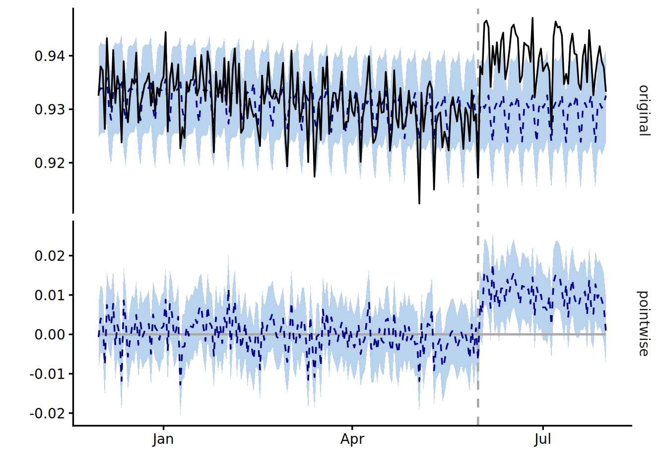
In the top panel of Figure 1, the observed outcome rises above the counterfactual after release. The interval width in the bottom panel remains nearly constant across the 61 days. The local-level innovation \(\sigma_\eta\) is small relative to the observation noise, so the additional variance from the longer forecast horizon is not visually prominent. Pointwise-effect intervals are wider than the interval for the average effect because they include daily binomial noise, whose standard deviation is about 0.4 pp. The purpose of this figure is not to classify individual days as having an effect, but to assess whether the effect persists across the period.
The spike-and-slab prior has an expected model size of 3, giving each of the 10 control series a prior inclusion probability of 30%.
| Control series | With weekly seasonality | Without seasonality (default) |
|---|---|---|
| android | 5.4% | 99.7% |
| mobile-web | 0.9% | 28.4% |
| android-tv | 2.2% | 11.6% |
| smart-tv-c | 0.6% | 6.1% |
| smart-tv-a | 0.6% | 4.6% |
| streaming-stick | 0.5% | 4.5% |
| game-console | 1.0% | 2.9% |
| smart-tv-b | 0.4% | 0.6% |
| tv-web | 0.3% | 0.5% |
| pc-web | 0.4% | 0.3% |
Table 2 reports the posterior inclusion probabilities of the regression coefficients. In the model with weekly seasonality, every control series has a posterior inclusion probability well below its 30% prior probability.
This result is consistent with the data-generating process. The weekly cycle and trend are the only features shared across devices; daily binomial noise is independent across devices. Once the weekly component and local level capture the shared structure, little variation remains for the control series to explain. Without a seasonal component, by contrast, Android receives a relatively high inclusion probability because the regression component takes over the task of capturing the weekly cycle.
SCM must use the controls because it constructs a convex combination. BSTS selects a control only when there is shared variation that the state components cannot explain. If posterior inclusion probabilities are also low in real data, the control series contribute little to the counterfactual forecast. The counterfactual should then be understood primarily as an extension of the treated unit’s own pre-treatment trend and seasonality into the post-treatment period.
Comparing the methods
I compare the three methods over the same 61-day post-treatment period. The DiD article used a seven-day window to match an operational decision horizon; here I recompute the same estimator over 61 days. The SCM estimate comes from the corresponding article.
| Method | Estimate | Lower | Upper | Interval construction | Assumption supporting the counterfactual |
|---|---|---|---|---|---|
| DiD (61-day window) | 1.155 | 0.945 | 1.366 | 95% CI from an asymptotic normal approximation to the binomial variance | Parallel trends |
| SCM | 1.08 | — | — | None (rank from in-space placebos, p = 1/11) | The pre-treatment factor structure persists after treatment |
| CausalImpact | 1.006 | 0.836 | 1.178 | 95% posterior interval from posterior prediction of the counterfactual | The state structure and relationship with the controls remain stable across treatment |
All three point estimates are close to the true effect, but that is because the data-generating process was designed to satisfy each method’s assumptions. With real data, we cannot verify whether parallel trends, persistence of the factor structure, or stability of the relationship with the controls continues to hold in the post-treatment period. Pre-treatment trends and model fit provide useful evidence, but they do not prove these assumptions.
In this application in particular, the CausalImpact estimate depends more heavily on the assumption that the pre-treatment iOS trend and weekly cycle continue after treatment than on the relationship between iOS and the control series.
The inferential statements also differ across methods. DiD provides a confidence interval based on an asymptotic normal approximation to the binomial variance; SCM produces a rank in increments of \(1/11\); and CausalImpact provides a posterior interval conditional on the model and priors. What the methods share is that each constructs a counterfactual from assumptions that cannot be verified directly. BSTS combines the treated unit’s own temporal structure with control series and expresses uncertainty about the counterfactual through a posterior predictive interval. That interval is conditional on the model and priors, however, and does not by itself guarantee the validity of the causal effect. When interpreting the estimate, it is essential to identify which components support the counterfactual and to state explicitly the assumption that those components remain stable after treatment.
R code
library(tidyverse)

date_treat <- lubridate::ymd("2026-06-01")
att_true <- 0.01049

panel <- read_csv("panel_parallel.csv")

# Replace hyphens in device names because they are awkward to use in formulas.
# Column 1 is the date, column 2 is the treated unit (iOS), and the rest are the 10 controls.
rates <- panel |>
  mutate(device = str_replace_all(device, "-", "_")) |>
  pivot_wider(
    id_cols = date,
    names_from = device,
    values_from = complete_rate
  ) |>
  arrange(date) |>
  relocate(date, ios) # Column 1: date; column 2: outcome y (iOS)

pre_period <- lubridate::ymd(c("2025-12-01", "2026-05-31"))
post_period <- lubridate::ymd(c("2026-06-01", "2026-07-31"))

# --- Local level + weekly seasonality + regression (CausalImpact internally fixes the seed at 1) ---

impact <- CausalImpact::CausalImpact(
  rates,
  pre.period = pre_period,
  post.period = post_period,
  model.args = list(nseasons = 7, niter = 5000)
)

# Average post-treatment effect and 95% posterior interval; omit the cumulative-effect row
impact$summary["Average", c("AbsEffect", "AbsEffect.lower", "AbsEffect.upper")]

# Observed and counterfactual series above; pointwise effect below; omit the cumulative-effect panel
plot(impact, c("original", "pointwise"))

# --- Reference: default model without a seasonal component ---

impact_noseason <- CausalImpact::CausalImpact(
  rates,
  pre.period = pre_period,
  post.period = post_period,
  model.args = list(niter = 5000)
)

# Posterior inclusion probabilities after removing the burn-in suggested from the log likelihood
coef_draws <- function(fit, model_name) {
  burn <- bsts::SuggestBurn(0.1, fit$model$bsts.model)

  fit$model$bsts.model$coefficients[-seq_len(burn), , drop = FALSE] |>
    as_tibble() |>
    mutate(model = model_name, draw = row_number(), .before = 1)
}

bind_rows(
  coef_draws(impact, "seasonal"),
  coef_draws(impact_noseason, "noseason")
) |>
  pivot_longer(-c(model, draw), names_to = "series", values_to = "beta") |>
  filter(series != "(Intercept)") |>
  summarise(inclusion = mean(beta != 0), .by = c(model, series))

# --- Comparison: recompute DiD (iOS versus Android) over a 61-day post-treatment window ---

panel |>
  filter(device %in% c("ios", "android")) |>
  mutate(period = if_else(post, "post", "pre")) |>
  summarise(
    complete = sum(complete),
    impression = sum(impression),
    .by = c(device, period)
  ) |>
  mutate(
    rate = complete / impression,
    var_rate = rate * (1 - rate) / impression
  ) |>
  pivot_wider(
    names_from = period,
    values_from = c(rate, var_rate),
    id_cols = device
  ) |>
  mutate(
    diff = rate_post - rate_pre,
    var_diff = var_rate_post + var_rate_pre,
    .keep = "unused"
  ) |>
  pivot_wider(names_from = device, values_from = c(diff, var_diff)) |>
  mutate(
    estimate = diff_ios - diff_android,
    se = sqrt(var_diff_ios + var_diff_android),
    ci_lower = estimate - qnorm(0.975) * se,
    ci_upper = estimate + qnorm(0.975) * se,
    .keep = "none"
  )