| donor | \(w_j\) |
|---|---|
| android | 0.408 |
| pc-web | 0.158 |
| mobile-web | 0.120 |
| smart-tv-b | 0.081 |
| game-console | 0.051 |
| smart-tv-a | 0.040 |
| tv-web | 0.038 |
| android-tv | 0.037 |
| streaming-stick | 0.033 |
| smart-tv-c | 0.033 |
The previous article estimated the effect of the ad pause feature, released on iOS only, with difference-in-differences (DiD from here on). The 7-day-window estimate with Android as the control was +1.31 percentage points (pp from here on), and the 95% CI covered the true treatment effect, the ATT (average treatment effect on the treated) of +1.049pp.
The problem that remains is the choice of the control. Android was chosen for three reasons: the conditions on the control group, the closeness of the confounding structure, and volume. All three are the analyst’s qualitative judgments, with no backing from the data. There are 10 candidate devices, and picking one is arbitrary; averaging all 10 with equal weights is arbitrary too.
The synthetic control method (SCM from here on) lets the data decide the weights on the controls. The criterion is how well the pre-period is reproduced: build the weighted average of the controls that best reproduces the pre-treatment iOS series, and after the treatment, use it as a stand-in for the iOS of the world without the treatment.
This article does the following three things:
- Define the SCM estimator, and lay out what the constraint on the weights demands, together with the correspondence to DiD.
- Estimate the weights with {tidysynth}, check their allocation and the pre-period fit, then compare the average gap over the 61 post-period days against the true +1.049pp.
- Run inference with the in-space placebo test, and confirm its limitation: the resolution of the p-value is capped by the number of control candidates.
The procedure is restricted to the standard form of Abadie, Diamond, and Hainmueller (2010): estimate the weights, check the gap, and rank with the in-space placebo. The implementation uses {tidysynth} as is. This article does not go into extensions that allow an intercept or extrapolation, such as augmented SCM.
The SCM estimator
The 10 control devices are called donors. Write \(Y_{jt}\) for the completion rate of donor \(j\) on day \(t\) (\(j = 1, \dots, J\), \(J = 10\)), and \(Y_{\text{iOS},t}\) for the completion rate of iOS. The synthetic control is built as a convex combination of the donors, that is, a weighted average with weights \(w_j\) that are non-negative and sum to one.
\[ \hat{Y}^{\text{synth}}_{t} = \sum_{j=1}^{J} w_j\, Y_{jt}, \qquad w_j \geq 0, \quad \sum_{j=1}^{J} w_j = 1 \]
The weights \(w_j\) are chosen by how well they reproduce the pre-period iOS series. Write \(T\) for the release date and \(T_{\text{pre}}\) for the number of pre-period days (182 in this data). The criterion is the pre-period mean squared prediction error (MSPE from here on),
\[ \frac{1}{T_{\text{pre}}} \sum_{t<T} \left( Y_{\text{iOS},t} - \sum_{j} w_j\, Y_{jt} \right)^2 \]
minimized under the convex-combination constraint.
For each post-treatment day, the difference between the observed iOS value \(Y_{\text{iOS},t}\) and the synthetic control \(\hat{Y}^{\text{synth}}_t\), the gap, is the estimate of that day’s effect.
\[ \hat{\tau}_t = Y_{\text{iOS},t} - \hat{Y}^{\text{synth}}_t \qquad (t \geq T) \]
The ATT estimate is the simple average of \(\hat{\tau}_t\) over the post-period.
Reading this gap as the effect takes two conditions. One is that the conditions on the control group placed in the DiD article hold for all 10 donors: every donor is untreated and free of spillover from the treatment. A path by which a UI change inside the iOS app spills over into the completion rate of another device is hard to imagine, so the judgment made for Android alone carries over to all 10. The other is that the pre-period is not contaminated by anticipation of the treatment (no anticipation). Since the weights are chosen to reproduce the pre-period, if the pre-period already contains the effect of the treatment, reproducing it no longer reproduces the counterfactual. The UI feature here is invisible to users until release, so this concern does not apply either.
The correspondence with DiD
With only one donor, the constraints force its weight to 1, and the synthetic control is that donor’s series itself. In other words, the Android series that the DiD article used as the control is, from SCM’s point of view, the special case of a single donor. The estimators, however, are not the same. The table below lays out the differences.
| DiD | SCM | |
|---|---|---|
| Control series | Android alone, chosen by the analyst | A convex combination of 10 donors, weights decided by the data |
| Handling of level differences | Cancels the moment the pre-post difference is taken | Not subtracted away; the level itself is reproduced |
| Pre-period information | A single point, the pre-period mean | The entire daily series |
| Assumption behind the counterfactual | Parallel trends | The factor structure that reproduced the pre-period persists post |
The essential difference is the handling of level differences. The SCM formulation has no intercept term, so a level difference stays in the gap as is. Indeed, restricting the donor to Android alone gives an average gap of +2.20pp over the 61 post-period days, exceeding the true +1.049pp by the pre-existing level difference of about +1pp.
With no intercept to absorb it, the synthetic control must reproduce the level itself. At each time point, a convex combination stays between the minimum and the maximum of the donors; it cannot extrapolate. Reproducing the level is therefore possible only when the treated unit’s level lies inside that range, the convex hull. Placing the iOS level inside the convex hull of the controls in the article that designed the synthetic data was the groundwork for exactly this. The iOS pre-period level of 93.1% sits inside the control range of 91.5 to 97.1%.
Estimating the weights
{tidysynth} takes, as the input that determines the weights, aggregates called predictors. The predictors here are the pre-period monthly mean completion rates (six values, 2025-12 through 2026-05); a month is the aggregation unit that smooths out the daily noise and the weekly cycle while keeping the shape of the level and the trend. The optimization window is the full 182-day pre-period. Internally the optimization is two-staged, with weights over the predictors (Abadie, Diamond, and Hainmueller 2010), but the final criterion for choosing the weights is still the MSPE of the previous section, so this article does not go into the details of that formulation.
Table 1 shows the estimated weights. The largest is android at 0.41, followed by pc-web at 0.16 and mobile-web at 0.12, and the remaining seven devices each get a small weight of 0.03 to 0.08.
This allocation can be explained from the generating process. Devices differ only in level and independent noise; the weekly cycle and the shape of the common trend are shared by all of them. All the synthetic control has to do, then, is reproduce the iOS level, so the weights should split between donors below the iOS level and donors above it. Indeed, the three devices below iOS (android, pc-web, and smart-tv-b) carry a total weight of 0.65 and the seven above it 0.35, and the weighted average of the pre-period levels is 93.1%, matching the iOS pre-period level. The weights spread widely instead of concentrating on a single device because the binomial noise, independent across units, averages out and lowers the pre-period MSPE by that much.
The gap and the estimate
The post-period window uses all 61 generated days. In a decision-making setting, the answer would come after 7 days, as in the DiD article. The interest of this article, though, is not the decision but evaluating how well SCM reproduces the counterfactual against the true value, and that evaluation is better served by more post-period observations.
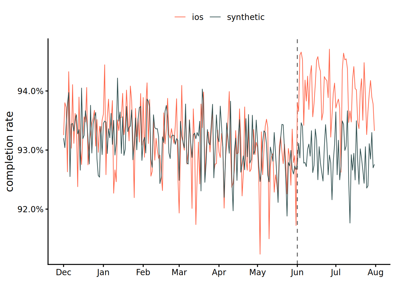
Figure 1 overlays the observed series and the synthetic control. The two lines are nearly indistinguishable in the pre-period, and the observed series pulls away upward at the release date.
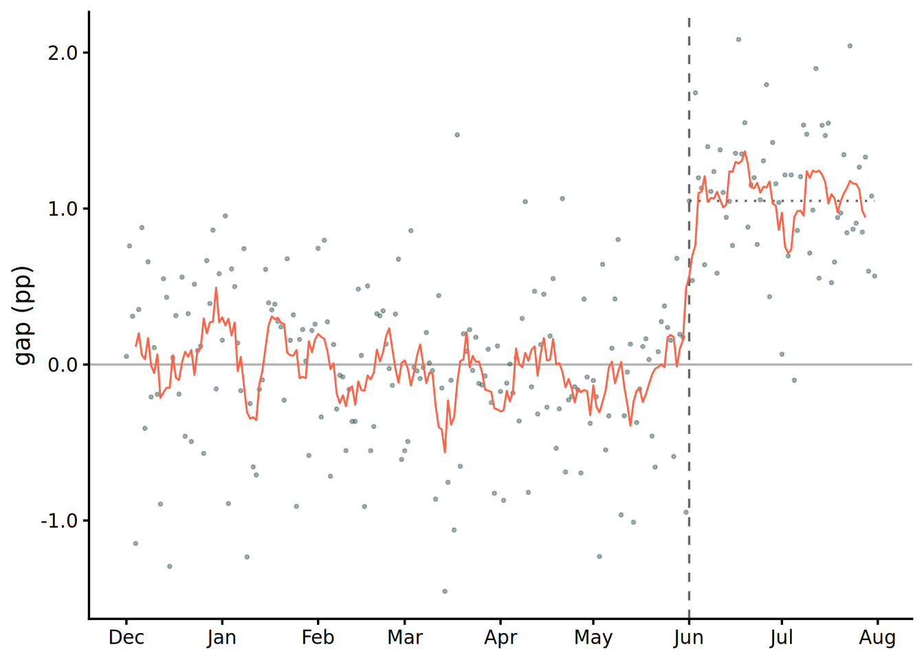
The gap in Figure 2, the difference of the two, is easier to read. The pre-period gap has a mean of −0.03pp and a root mean squared error (RMSE) of 0.52pp, and the 7-day moving average hugs zero. At the release date the moving average lifts to a little over +1pp; the average gap over the 61 post-period days is +1.08pp, and the difference from the true +1.049pp is +0.03pp.
The point estimate is in hand. The next question is whether this +1.08pp is more than chance.
Inference with the in-space placebo
In DiD, a CI could be built by computing the standard error from the binomial variances of the four completion rates, split by group and period. SCM does not allow the same, because no closed-form expression exists for the standard error of the point estimate. There are two reasons. One is that the weights solve an optimization under the inequality constraints of non-negativity and summing to one, so the solution can sit on the boundary of the constraints (some \(w_j\) exactly 0), making the estimator a non-smooth function of the data. The other is that with a single treated unit and a fixed donor pool, the very framework of asymptotics, what is sent to infinity, is not defined (Abadie 2021).
The standard alternative is the in-space placebo test. The null distribution of the gap cannot be derived analytically, so the same procedure is run on units known to have zero effect, and the distribution is built empirically.
For example, treat android as the unit treated on 2026-06-01, take the remaining 10 devices as its donors (in the {tidysynth} implementation this includes iOS), estimate the weights with the same predictors and the same window, and compute the gap series. No treatment exists for android, so this gap is what the procedure outputs when the effect is zero. Repeating the same computation for all 10 donors yields one iOS gap and 10 placebo gaps. If the treatment is real, only the iOS gap should break away from this bundle.
The iOS post-period on the donor side does contain the actual treatment, but on average that contamination inflates the placebo post-period MSPE, working against iOS in the ranking.
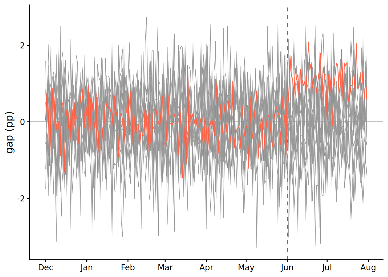
One caution when reading Figure 3: the sizes of the post-period gaps must not be compared as they are. A donor whose level sits near the edge of the convex hull (smart-tv-b, the lowest, for instance) is hard to reproduce as a convex combination of the remaining units, and its gap is large from the pre-period on. A unit that does not fit before the treatment will not fit after it either, and that is no evidence of a treatment.
The test statistic is therefore the ratio of the post-period MSPE to the pre-period MSPE. A unit with a poor fit from the start has a large denominator too, so its ratio does not inflate. Sort the ratios of all 11 units in descending order, and the rank of the treated unit gives the p-value.
\[ p = \frac{\text{rank}}{J + 1} \]
This is the exact p-value of a permutation test, under the view that the treatment could just as well have landed on any of the 11 units.
| unit | Pre MSPE | Post MSPE | Ratio | Rank | \(p\) |
|---|---|---|---|---|---|
| ios | 0.27 | 1.36 | 5.08 | 1 | 0.091 |
| android | 0.63 | 0.87 | 1.39 | 2 | 0.182 |
| streaming-stick | 0.74 | 1.02 | 1.38 | 3 | 0.273 |
| mobile-web | 1.14 | 1.44 | 1.25 | 4 | 0.364 |
| smart-tv-b | 1.39 | 1.69 | 1.21 | 5 | 0.455 |
| smart-tv-c | 0.67 | 0.77 | 1.16 | 6 | 0.545 |
| smart-tv-a | 0.51 | 0.57 | 1.13 | 7 | 0.636 |
| tv-web | 0.67 | 0.72 | 1.08 | 8 | 0.727 |
| android-tv | 0.49 | 0.51 | 1.05 | 9 | 0.818 |
| game-console | 1.24 | 1.15 | 0.93 | 10 | 0.909 |
| pc-web | 0.87 | 0.80 | 0.93 | 11 | 1.000 |
The iOS ratio is 5.08, rank 1, far ahead of android in second place at 1.39. The p-value is \(1/11 \approx 0.091\).
Here lies the limit of resolution. With 10 donors, no matter how clear the effect, the p-value cannot go below \(1/11\). The 5% level is out of reach in principle, and what sets the granularity of the p-value is the number of donors, not the strength of the effect. Reading this test as a ranking, showing where the treated unit’s gap stands in the placebo distribution, matches what it actually does better than reading it as a significance verdict.
Only the pre-period can be verified
What SCM lets you check is only how well the pre-period was reproduced. Reading the post-period gap as the effect requires the assumption that the factor structure behind the pre-period fit continues into the post-period. That is a claim about the post-period counterfactual, so it cannot be verified. Its standing is the same as the parallel trends assumption in DiD: removing the arbitrariness from the choice of the control does not change the fact that the counterfactual is built out of an assumption.
A good pre-period fit is no proof of this assumption. With enough donors, the pre-period can be reproduced by overfitting to noise. In the data of this article, the generating process itself guarantees that all units share the same day-of-week and trend structure and that this does not change in the post-period. Real data comes with no such guarantee. Being able to check how a method behaves on synthetic data and being able to check the assumption on real data are two different things.
Inference without an interval
What this article obtained is a point estimate within +0.03pp of the true value and a rank of 1 by the MSPE ratio. The expression of uncertainty, however, stops at a rank-based p-value; there is no continuous interval comparable to the CI that DiD could build. Inference that gives SCM an interval has been proposed in several forms, starting with conformal inference based on permutations along the time dimension (Chernozhukov, Wüthrich, and Zhu 2021), but all of them lie outside the standard procedure this article restricted itself to at the start. Modeling the time structure explicitly and producing the counterfactual prediction with its interval directly is the approach of CausalImpact, the subject of the next article.
R code
The whole analysis can be reproduced just by reading panel_parallel.csv, the output of the generator in the article that designed the synthetic data.
library(tidyverse)

date_treat <- lubridate::ymd("2026-06-01")

panel <- read_csv("panel_parallel.csv")

# SCM: predictors are the pre-period monthly means;
# the optimization window is the full pre-period.
# tidysynth treats time <= i_time as the pre-period,
# so pass the day before the release as i_time
sc <- panel |>
  tidysynth::synthetic_control(
    outcome = complete_rate,
    unit = device,
    time = date,
    i_unit = "ios",
    i_time = date_treat - 1,
    generate_placebos = TRUE
  ) |>
  tidysynth::generate_predictor(
    time_window = seq(
      lubridate::ymd("2025-12-01"),
      lubridate::ymd("2025-12-31"),
      by = "day"
    ),
    rate_2025_12 = mean(complete_rate)
  ) |>
  tidysynth::generate_predictor(
    time_window = seq(
      lubridate::ymd("2026-01-01"),
      lubridate::ymd("2026-01-31"),
      by = "day"
    ),
    rate_2026_01 = mean(complete_rate)
  ) |>
  tidysynth::generate_predictor(
    time_window = seq(
      lubridate::ymd("2026-02-01"),
      lubridate::ymd("2026-02-28"),
      by = "day"
    ),
    rate_2026_02 = mean(complete_rate)
  ) |>
  tidysynth::generate_predictor(
    time_window = seq(
      lubridate::ymd("2026-03-01"),
      lubridate::ymd("2026-03-31"),
      by = "day"
    ),
    rate_2026_03 = mean(complete_rate)
  ) |>
  tidysynth::generate_predictor(
    time_window = seq(
      lubridate::ymd("2026-04-01"),
      lubridate::ymd("2026-04-30"),
      by = "day"
    ),
    rate_2026_04 = mean(complete_rate)
  ) |>
  tidysynth::generate_predictor(
    time_window = seq(
      lubridate::ymd("2026-05-01"),
      lubridate::ymd("2026-05-31"),
      by = "day"
    ),
    rate_2026_05 = mean(complete_rate)
  ) |>
  tidysynth::generate_weights(
    optimization_window = seq(
      lubridate::ymd("2025-12-01"),
      lubridate::ymd("2026-05-31"),
      by = "day"
    )
  ) |>
  tidysynth::generate_control()

# donor weights
sc |>
  tidysynth::grab_unit_weights() |>
  arrange(desc(weight))
#> unit            weight
#> android         0.408
#> pc-web          0.158
#> mobile-web      0.120
#> smart-tv-b      0.0806
#> game-console    0.0505
#> smart-tv-a      0.0401
#> tv-web          0.0385
#> android-tv      0.0372
#> streaming-stick 0.0333
#> smart-tv-c      0.0331

# pre-period fit and the post-period mean gap
sc |>
  tidysynth::grab_synthetic_control() |>
  mutate(period = if_else(time_unit >= date_treat, "post", "pre")) |>
  summarise(
    rmse = sqrt(mean((real_y - synth_y)^2)),
    gap = mean(real_y - synth_y),
    .by = period
  )
#> period     rmse        gap
#> pre     0.00517  -0.000309
#> post    0.0116    0.0108

# in-space placebo: MSPE-ratio ranks and p-values
sc |>
  tidysynth::grab_significance() |>
  select(unit_name, pre_mspe, post_mspe, mspe_ratio, rank, fishers_exact_pvalue)
#> unit_name        pre_mspe   post_mspe  mspe_ratio  rank  fishers_exact_pvalue
#> ios              0.0000267  0.000136        5.08      1                0.0909
#> android          0.0000628  0.0000872       1.39      2                0.182
#> streaming-stick  0.0000737  0.000102        1.38      3                0.273
#> (rest omitted; the 10 donor ratios fall between 0.93 and 1.39)

# restricting the donor to Android alone:
# the pre-existing level difference goes straight into the gap
panel |>
  filter(date >= date_treat, device %in% c("ios", "android")) |>
  pivot_wider(
    names_from = device,
    values_from = complete_rate,
    id_cols = date
  ) |>
  summarise(gap = mean(ios - android))
#> gap
#> 0.0220